Chapter 5 Key Concept The Definite Integral Section

Chapter 5 Key Concept: The Definite Integral Section 5. 1 How Do We Measure Distance Traveled? Section 5. 2 The Definite Integral Section 5. 3 The Fundamental Theorem and Interpretations Section 5. 4 Theorems About Definite Integrals Calculus, 6 th edition, Hughes-Hallett et. al. , Copyright 2013 by John Wiley & Sons, All Rights Reserved

Section 5. 1 How Do We Measure Distance Traveled? Calculus, 6 th edition, Hughes-Hallett et. al. , Copyright 2013 by John Wiley & Sons, All Rights Reserved

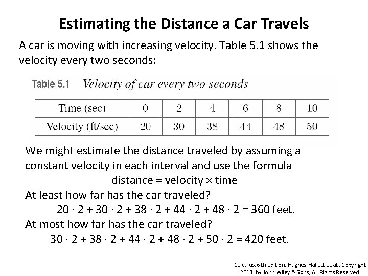
Estimating the Distance a Car Travels A car is moving with increasing velocity. Table 5. 1 shows the velocity every two seconds: We might estimate the distance traveled by assuming a constant velocity in each interval and use the formula distance = velocity × time At least how far has the car traveled? 20 · 2 + 38 · 2 + 44 · 2 + 48 · 2 = 360 feet. At most how far has the car traveled? ining the data 30 · 2 + 38 · 2 + 44 · 2 + 48 · 2 + 50 · 2 = 420 feet. 1: Calculus, 6 th edition, Hughes-Hallett et. al. , Copyright 2013 by John Wiley & Sons, All Rights Reserved

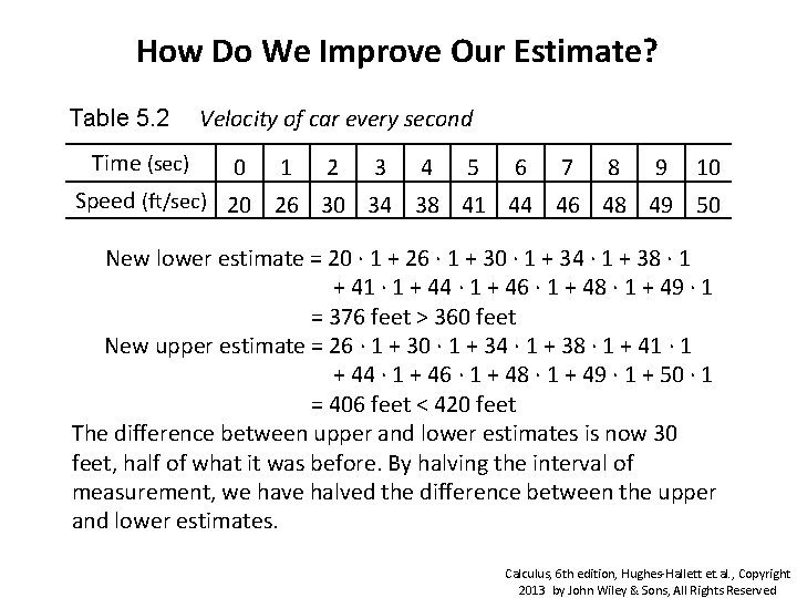
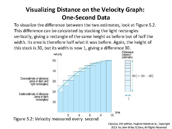
How Do We Improve Our Estimate? Table 5. 2 Time (sec) Velocity of car every second 0 1 2 3 4 5 6 7 8 9 10 Speed (ft/sec) 20 26 30 34 38 41 44 46 48 49 50 New lower estimate = 20 · 1 + 26 · 1 + 30 · 1 + 34 · 1 + 38 · 1 + 41 · 1 + 44 · 1 + 46 · 1 + 48 · 1 + 49 · 1 = 376 feet > 360 feet New upper estimate = 26 · 1 + 30 · 1 + 34 · 1 + 38 · 1 + 41 · 1 + 44 · 1 + 46 · 1 + 48 · 1 + 49 · 1 + 50 · 1 = 406 feet < 420 feet The difference between upper and lower estimates is now 30 feet, half of what it was before. By halving the interval of measurement, we have halved the difference between the upper and lower estimates. Calculus, 6 th edition, Hughes-Hallett et. al. , Copyright 2013 by John Wiley & Sons, All Rights Reserved

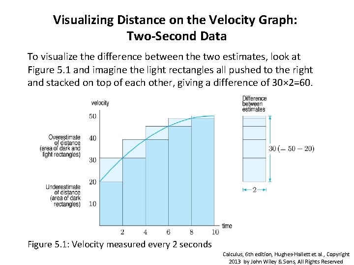
Visualizing Distance on the Velocity Graph: Two-Second Data To visualize the difference between the two estimates, look at Figure 5. 1 and imagine the light rectangles all pushed to the right and stacked on top of each other, giving a difference of 30× 2=60. Figure 5. 1: Velocity measured every 2 seconds Calculus, 6 th edition, Hughes-Hallett et. al. , Copyright 2013 by John Wiley & Sons, All Rights Reserved

Visualizing Distance on the Velocity Graph: One-Second Data To visualize the difference between the two estimates, look at Figure 5. 2. This difference can be calculated by stacking the light rectangles vertically, giving a rectangle of the same height as before but of half the width. Its area is therefore half what it was before. Again, the height of this stack is 30, but its width is now 1, giving a difference 30. Figure 5. 2: Velocity measured every second Calculus, 6 th edition, Hughes-Hallett et. al. , Copyright 2013 by John Wiley & Sons, All Rights Reserved

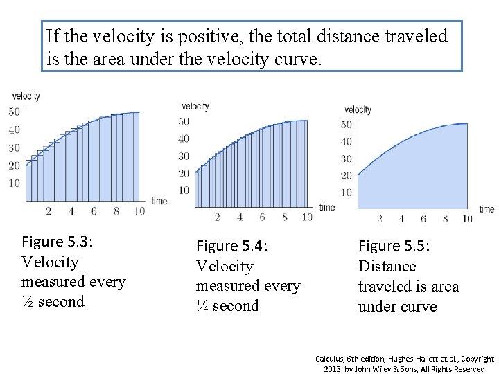
If the velocity is positive, the total distance traveled is the area under the velocity curve. Figure 5. 3: Velocity measured every ½ second Figure 5. 4: Velocity measured every ¼ second Figure 5. 5: Distance traveled is area under curve Calculus, 6 th edition, Hughes-Hallett et. al. , Copyright 2013 by John Wiley & Sons, All Rights Reserved

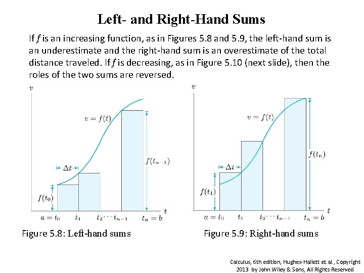
Left- and Right-Hand Sums If f is an increasing function, as in Figures 5. 8 and 5. 9, the left-hand sum is an underestimate and the right-hand sum is an overestimate of the total distance traveled. If f is decreasing, as in Figure 5. 10 (next slide), then the roles of the two sums are reversed. Figure 5. 8: Left-hand sums Figure 5. 9: Right-hand sums Calculus, 6 th edition, Hughes-Hallett et. al. , Copyright 2013 by John Wiley & Sons, All Rights Reserved

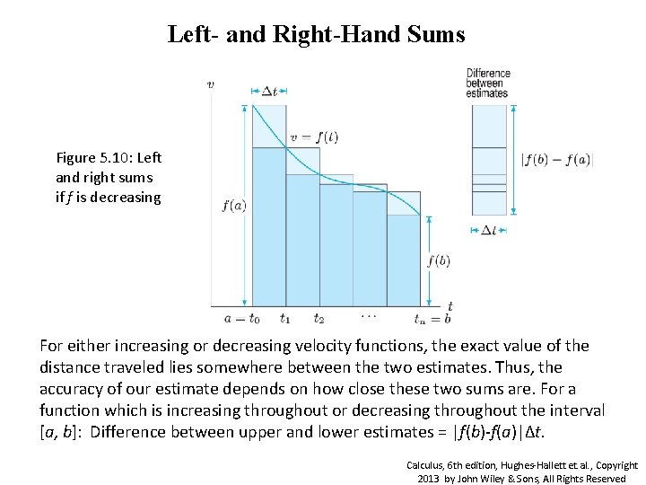
Left- and Right-Hand Sums Figure 5. 10: Left and right sums if f is decreasing For either increasing or decreasing velocity functions, the exact value of the distance traveled lies somewhere between the two estimates. Thus, the accuracy of our estimate depends on how close these two sums are. For a function which is increasing throughout or decreasing throughout the interval [a, b]: Difference between upper and lower estimates = |f(b)-f(a)|Δt. Calculus, 6 th edition, Hughes-Hallett et. al. , Copyright 2013 by John Wiley & Sons, All Rights Reserved

Section 5. 2 The Definite Integral Calculus, 6 th edition, Hughes-Hallett et. al. , Copyright 2013 by John Wiley & Sons, All Rights Reserved

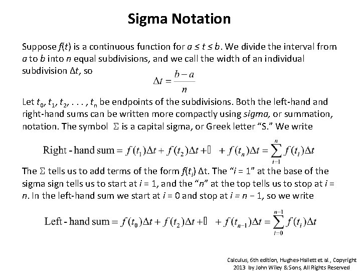
Sigma Notation Suppose f(t) is a continuous function for a ≤ t ≤ b. We divide the interval from a to b into n equal subdivisions, and we call the width of an individual subdivision Δt, so Let t 0, t 1, t 2, . . . , tn be endpoints of the subdivisions. Both the left-hand right-hand sums can be written more compactly using sigma, or summation, notation. The symbol Σ is a capital sigma, or Greek letter “S. ” We write The Σ tells us to add terms of the form f(ti) Δt. The “i = 1” at the base of the sigma sign tells us to start at i = 1, and the “n” at the top tells us to stop at i = n. In the left-hand sum we start at i = 0 and stop at i = n − 1, so we write Calculus, 6 th edition, Hughes-Hallett et. al. , Copyright 2013 by John Wiley & Sons, All Rights Reserved

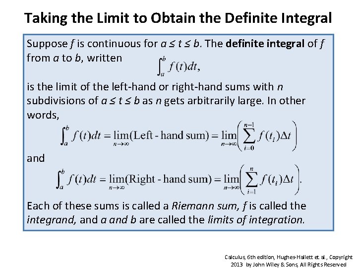
Taking the Limit to Obtain the Definite Integral Suppose f is continuous for a ≤ t ≤ b. The definite integral of f from a to b, written is the limit of the left-hand or right-hand sums with n subdivisions of a ≤ t ≤ b as n gets arbitrarily large. In other words, and Each of these sums is called a Riemann sum, f is called the integrand, and a and b are called the limits of integration. Calculus, 6 th edition, Hughes-Hallett et. al. , Copyright 2013 by John Wiley & Sons, All Rights Reserved

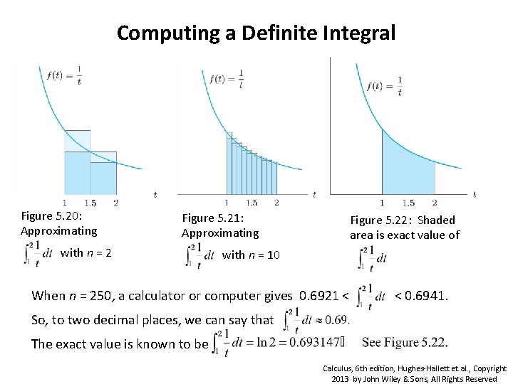
Computing a Definite Integral Figure 5. 20: Approximating Figure 5. 21: Approximating with n = 2 Figure 5. 22: Shaded area is exact value of with n = 10 When n = 250, a calculator or computer gives 0. 6921 < < 0. 6941. So, to two decimal places, we can say that The exact value is known to be Calculus, 6 th edition, Hughes-Hallett et. al. , Copyright 2013 by John Wiley & Sons, All Rights Reserved

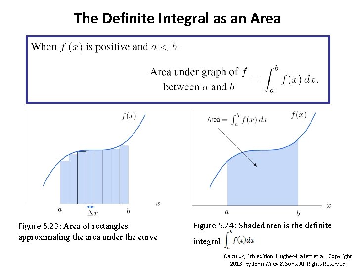
The Definite Integral as an Area Figure 5. 23: Area of rectangles approximating the area under the curve Figure 5. 24: Shaded area is the definite integral Calculus, 6 th edition, Hughes-Hallett et. al. , Copyright 2013 by John Wiley & Sons, All Rights Reserved

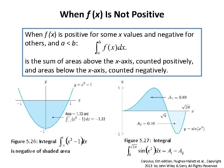
When f (x) Is Not Positive When f (x) is positive for some x values and negative for others, and a < b: is the sum of areas above the x-axis, counted positively, and areas below the x-axis, counted negatively. Figure 5. 26: Integral Figure 5. 27: Integral is negative of shaded area Calculus, 6 th edition, Hughes-Hallett et. al. , Copyright 2013 by John Wiley & Sons, All Rights Reserved

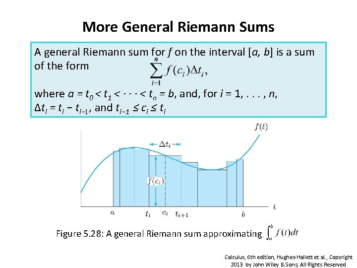
More General Riemann Sums A general Riemann sum for f on the interval [a, b] is a sum of the form where a = t 0 < t 1 < · · · < tn = b, and, for i = 1, . . . , n, Δti = ti − ti− 1, and ti− 1 ≤ ci ≤ ti Figure 5. 28: A general Riemann sum approximating Calculus, 6 th edition, Hughes-Hallett et. al. , Copyright 2013 by John Wiley & Sons, All Rights Reserved

Section 5. 3 The Fundamental Theorem and Interpretations Calculus, 6 th edition, Hughes-Hallett et. al. , Copyright 2013 by John Wiley & Sons, All Rights Reserved

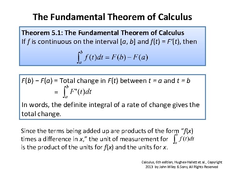
The Fundamental Theorem of Calculus Theorem 5. 1: The Fundamental Theorem of Calculus If f is continuous on the interval [a, b] and f(t) = F′(t), then F(b) − F(a) = Total change in F(t) between t = a and t = b = In words, the definite integral of a rate of change gives the total change. Since the terms being added up are products of the form “f(x) times a difference in x, ” the unit of measurement for is the product of the units for f(x) and the units for x. Calculus, 6 th edition, Hughes-Hallett et. al. , Copyright 2013 by John Wiley & Sons, All Rights Reserved

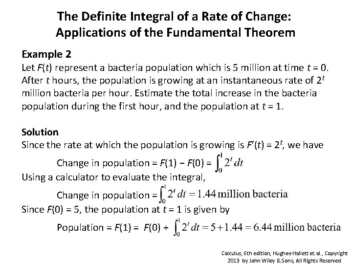
The Definite Integral of a Rate of Change: Applications of the Fundamental Theorem Example 2 Let F(t) represent a bacteria population which is 5 million at time t = 0. After t hours, the population is growing at an instantaneous rate of 2 t million bacteria per hour. Estimate the total increase in the bacteria population during the first hour, and the population at t = 1. Solution Since the rate at which the population is growing is F′(t) = 2 t, we have Change in population = F(1) − F(0) = Using a calculator to evaluate the integral, Change in population = Since F(0) = 5, the population at t = 1 is given by Population = F(1) = F(0) + Calculus, 6 th edition, Hughes-Hallett et. al. , Copyright 2013 by John Wiley & Sons, All Rights Reserved

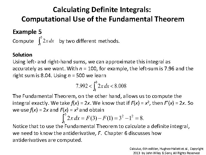
Calculating Definite Integrals: Computational Use of the Fundamental Theorem Example 5 Compute by two different methods. Solution Using left- and right-hand sums, we can approximate this integral as accurately as we want. With n = 100, for example, the left-sum is 7. 96 and the right sum is 8. 04. Using n = 500 we learn The Fundamental Theorem, on the other hand, allows us to compute the integral exactly. We take f(x) = 2 x. We know that if F(x) = x 2, then F′(x) = 2 x. So we use f(x) = 2 x and F(x) = x 2 and obtain Notice that to use the Fundamental Theorem to calculate a definite integral, we need to know the antiderivative, F. Chapter 6 discusses how antiderivatives are computed. Calculus, 6 th edition, Hughes-Hallett et. al. , Copyright 2013 by John Wiley & Sons, All Rights Reserved

Section 5. 4 Theorems About Definite Integrals Calculus, 6 th edition, Hughes-Hallett et. al. , Copyright 2013 by John Wiley & Sons, All Rights Reserved

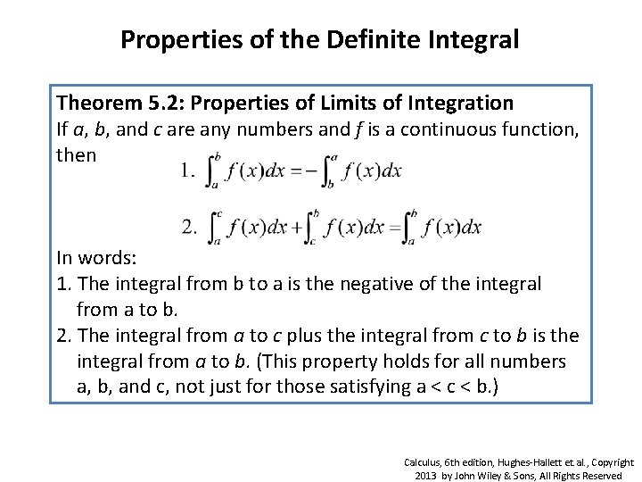
Properties of the Definite Integral Theorem 5. 2: Properties of Limits of Integration If a, b, and c are any numbers and f is a continuous function, then In words: 1. The integral from b to a is the negative of the integral from a to b. 2. The integral from a to c plus the integral from c to b is the integral from a to b. (This property holds for all numbers a, b, and c, not just for those satisfying a < c < b. ) Calculus, 6 th edition, Hughes-Hallett et. al. , Copyright 2013 by John Wiley & Sons, All Rights Reserved

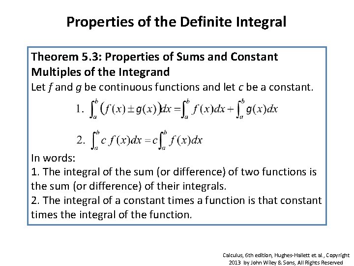
Properties of the Definite Integral Theorem 5. 3: Properties of Sums and Constant Multiples of the Integrand Let f and g be continuous functions and let c be a constant. In words: 1. The integral of the sum (or difference) of two functions is the sum (or difference) of their integrals. 2. The integral of a constant times a function is that constant times the integral of the function. Calculus, 6 th edition, Hughes-Hallett et. al. , Copyright 2013 by John Wiley & Sons, All Rights Reserved

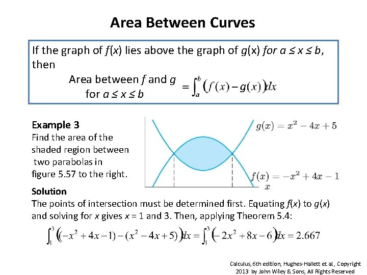
Area Between Curves If the graph of f(x) lies above the graph of g(x) for a ≤ x ≤ b, then Area between f and g for a ≤ x ≤ b Example 3 Find the area of the shaded region between two parabolas in figure 5. 57 to the right. Solution The points of intersection must be determined first. Equating f(x) to g(x) and solving for x gives x = 1 and 3. Then, applying Theorem 5. 4: Calculus, 6 th edition, Hughes-Hallett et. al. , Copyright 2013 by John Wiley & Sons, All Rights Reserved

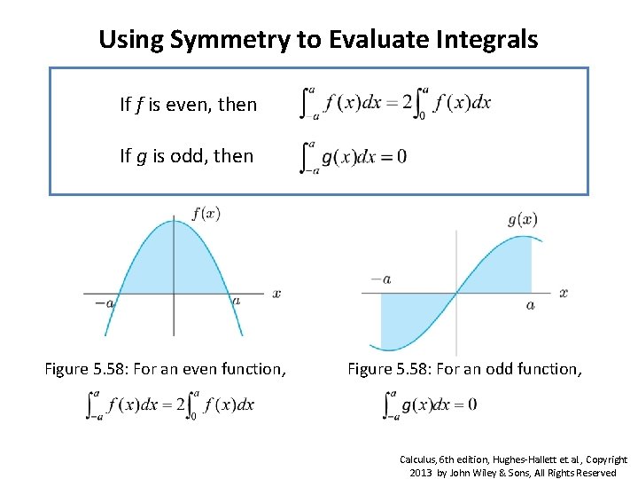
Using Symmetry to Evaluate Integrals If f is even, then If g is odd, then Figure 5. 58: For an even function, Figure 5. 58: For an odd function, Calculus, 6 th edition, Hughes-Hallett et. al. , Copyright 2013 by John Wiley & Sons, All Rights Reserved

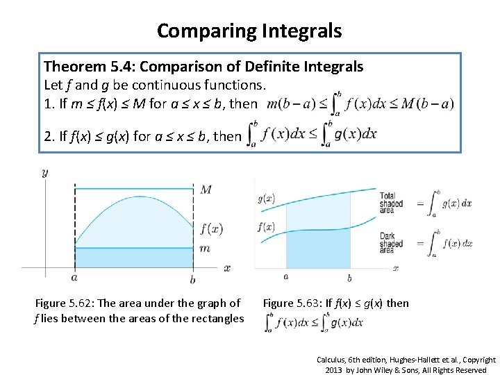
Comparing Integrals Theorem 5. 4: Comparison of Definite Integrals Let f and g be continuous functions. 1. If m ≤ f(x) ≤ M for a ≤ x ≤ b, then 2. If f(x) ≤ g(x) for a ≤ x ≤ b, then Figure 5. 62: The area under the graph of f lies between the areas of the rectangles Figure 5. 63: If f(x) ≤ g(x) then Calculus, 6 th edition, Hughes-Hallett et. al. , Copyright 2013 by John Wiley & Sons, All Rights Reserved

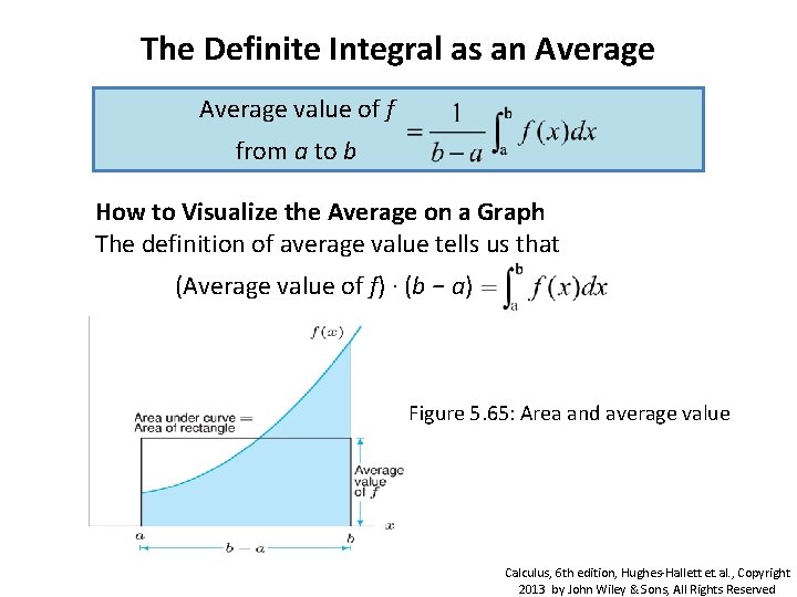
The Definite Integral as an Average value of f from a to b How to Visualize the Average on a Graph The definition of average value tells us that (Average value of f) · (b − a) Figure 5. 65: Area and average value Calculus, 6 th edition, Hughes-Hallett et. al. , Copyright 2013 by John Wiley & Sons, All Rights Reserved

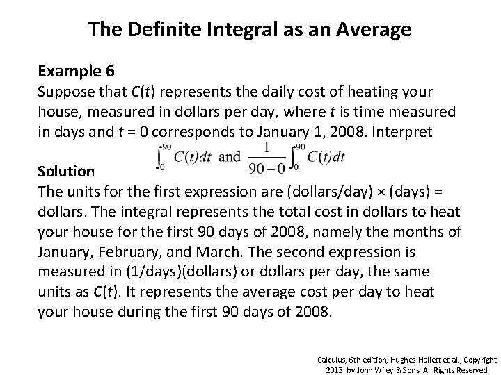
The Definite Integral as an Average Example 6 Suppose that C(t) represents the daily cost of heating your house, measured in dollars per day, where t is time measured in days and t = 0 corresponds to January 1, 2008. Interpret Solution The units for the first expression are (dollars/day) × (days) = dollars. The integral represents the total cost in dollars to heat your house for the first 90 days of 2008, namely the months of January, February, and March. The second expression is measured in (1/days)(dollars) or dollars per day, the same units as C(t). It represents the average cost per day to heat your house during the first 90 days of 2008. Calculus, 6 th edition, Hughes-Hallett et. al. , Copyright 2013 by John Wiley & Sons, All Rights Reserved