ASLevel Maths Statistics 1 for Edexcel S 1

AS-Level Maths: Statistics 1 for Edexcel S 1. 5 Discrete random variables These icons indicate that teacher’s notes or useful web addresses are available in the Notes Page. This icon indicates the slide contains activities created in Flash. These activities are not editable. For more detailed instructions, see the Getting Started presentation. 11 of of 39 39 © Boardworks Ltd 2005

Discrete random variables Introduction to discrete random variables Contents Cumulative distribution functions Expectation Variance and standard deviation for random variables Discrete uniform distribution Expectation algebra – some key results 22 of of 39 39 © Boardworks Ltd 2005

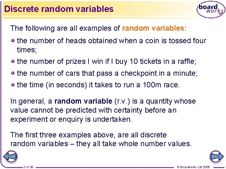
Discrete random variables The following are all examples of random variables: the number of heads obtained when a coin is tossed four times; the number of prizes I win if I buy 10 tickets in a raffle; the number of cars that pass a checkpoint in a minute; the time (in seconds) it takes to run a 100 m race. In general, a random variable (r. v. ) is a quantity whose value cannot be predicted with certainty before an experiment or enquiry is undertaken. The first three examples above, are all discrete random variables – they all take whole number values. 3 of 39 © Boardworks Ltd 2005

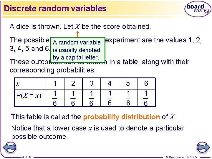
Discrete random variables A dice is thrown. Let X be the score obtained. The possible outcomes of this experiment are the values 1, 2, A random variable 3, 4, 5 and 6. is usually denoted by a capital letter. These outcomes can be shown in a table, along with their corresponding probabilities: 1 x 2 3 4 5 6 P(X = x) This table is called the probability distribution of X. Notice that a lower case x is used to denote a particular possible outcome. 4 of 39 © Boardworks Ltd 2005

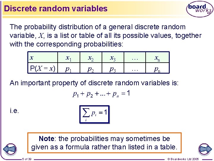
Discrete random variables The probability distribution of a general discrete random variable, X, is a list or table of all its possible values, together with the corresponding probabilities: x x 1 x 2 x 3 … xn P(X = x) p 1 p 2 p 3 … pn An important property of discrete random variables is: i. e. Note: the probabilities may sometimes be given as a formula rather than listed in a table. 5 of 39 © Boardworks Ltd 2005

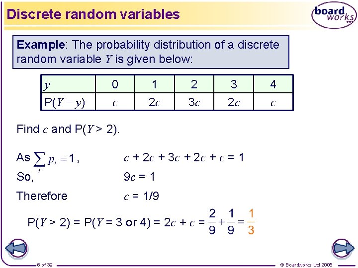
Discrete random variables Example: The probability distribution of a discrete random variable Y is given below: y P(Y = y) 0 c 1 2 c 2 3 c 3 2 c 4 c Find c and P(Y > 2). As , c + 2 c + 3 c + 2 c + c = 1 So, 9 c = 1 Therefore c = 1/9 P(Y > 2) = P(Y = 3 or 4) = 2 c + c = 6 of 39 © Boardworks Ltd 2005

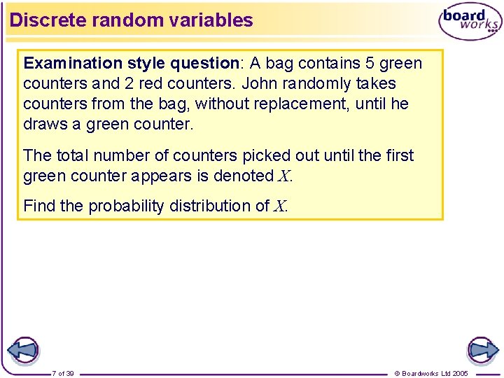
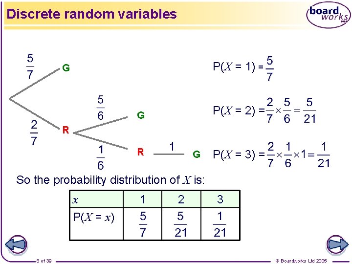
Discrete random variables Examination style question: A bag contains 5 green counters and 2 red counters. John randomly takes counters from the bag, without replacement, until he draws a green counter. The total number of counters picked out until the first green counter appears is denoted X. Find the probability distribution of X. 7 of 39 © Boardworks Ltd 2005

Discrete random variables P(X = 1) = G P(X = 2) = G R R 1 G P(X = 3) = So the probability distribution of X is: x P(X = x) 8 of 39 1 2 3 © Boardworks Ltd 2005

Cumulative distribution functions Introduction to discrete random variables Contents Cumulative distribution functions Expectation Variance and standard deviation for random variables Discrete uniform distribution Expectation algebra – some key results 99 of of 39 39 © Boardworks Ltd 2005

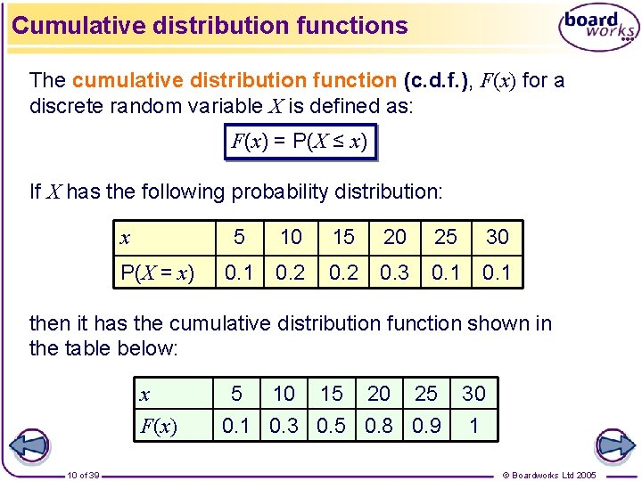
Cumulative distribution functions The cumulative distribution function (c. d. f. ), F(x) for a discrete random variable X is defined as: F(x) = P(X ≤ x) If X has the following probability distribution: x P(X = x) 5 10 15 20 25 30 0. 1 0. 2 0. 3 0. 1 then it has the cumulative distribution function shown in the table below: x F(x) 10 of 39 5 10 15 20 25 30 0. 1 0. 3 0. 5 0. 8 0. 9 1 © Boardworks Ltd 2005

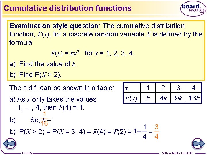
Cumulative distribution functions Examination style question: The cumulative distribution function, F(x), for a discrete random variable X is defined by the formula F(x) = kx 2 for x = 1, 2, 3, 4. a) Find the value of k. b) Find P(X > 2). The c. d. f. can be shown in a table: a) As x only takes the values 1, …, 4, then F(4) = 1. b) x F(x) 1 k 2 4 k 3 4 9 k 16 k So, k = b) P(X > 2) = P(X = 3, 4) = F(4) – F(2) = 11 of 39 © Boardworks Ltd 2005

Expectation Introduction to discrete random variables Contents Cumulative distribution functions Expectation Variance and standard deviation for random variables Discrete uniform distribution Expectation algebra – some key results 12 of 39 © Boardworks Ltd 2005

Gambling games 13 of 39 © Boardworks Ltd 2005

Gambling games 14 of 39 © Boardworks Ltd 2005

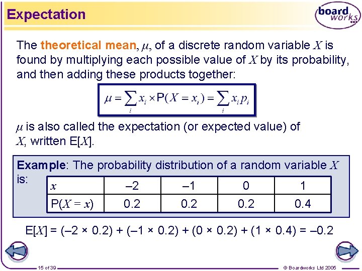
Expectation The theoretical mean, μ, of a discrete random variable X is found by multiplying each possible value of X by its probability, and then adding these products together: μ is also called the expectation (or expected value) of X, written E[X]. Example: The probability distribution of a random variable X is: x – 2 – 1 0 1 P(X = x) 0. 2 0. 4 E[X] = (– 2 × 0. 2) + (– 1 × 0. 2) + (0 × 0. 2) + (1 × 0. 4) = – 0. 2 15 of 39 © Boardworks Ltd 2005

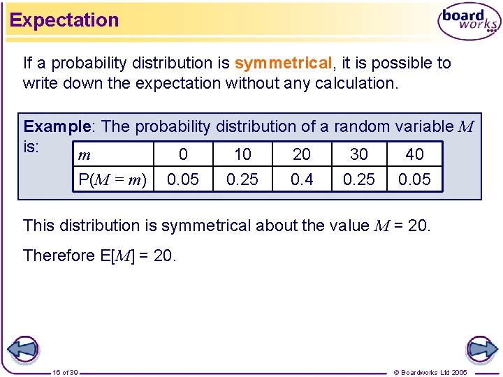
Expectation If a probability distribution is symmetrical, it is possible to write down the expectation without any calculation. Example: The probability distribution of a random variable M is: m 0 10 20 30 40 P(M = m) 0. 05 0. 25 0. 4 0. 25 0. 05 This distribution is symmetrical about the value M = 20. Therefore E[M] = 20. 16 of 39 © Boardworks Ltd 2005

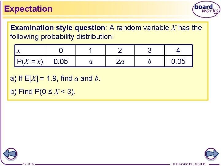
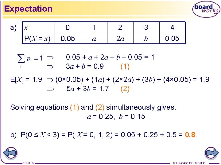
Expectation Examination style question: A random variable X has the following probability distribution: x P(X = x) 0 0. 05 1 a 2 2 a 3 b 4 0. 05 a) If E[X] = 1. 9, find a and b. b) Find P(0 ≤ X < 3). 17 of 39 © Boardworks Ltd 2005

Expectation a) x P(X = x) 0 0. 05 1 a 2 2 a 3 b 4 0. 05 + a + 2 a + b + 0. 05 = 1 3 a + b = 0. 9 (1) E[X] = 1. 9 (0× 0. 05) + (1 a) + (2× 2 a) + (3 b) + (4× 0. 05) = 1. 9 5 a + 3 b = 1. 7 (2) Solving equations (1) and (2) simultaneously gives: a = 0. 25, b = 0. 15 b) P(0 ≤ X < 3) = P( X = 0, 1, 2) = 0. 05 + 0. 25 + 0. 5 = 0. 8. 18 of 39 © Boardworks Ltd 2005

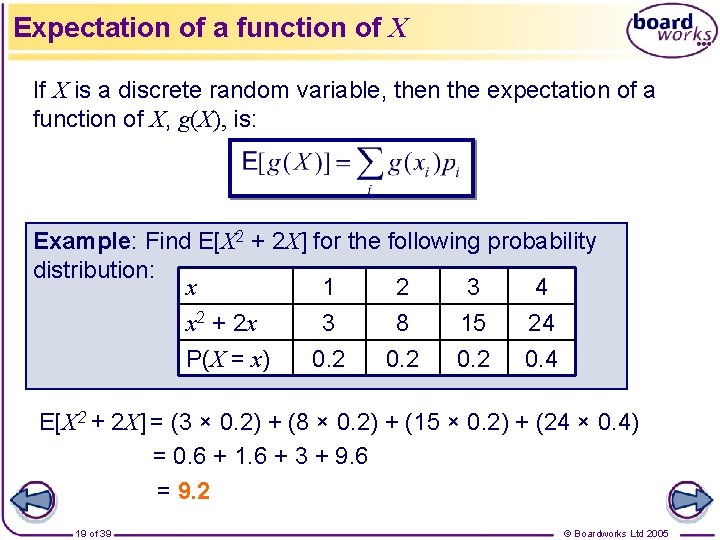
Expectation of a function of X If X is a discrete random variable, then the expectation of a function of X, g(X), is: Example: Find E[X 2 + 2 X] for the following probability distribution: x 1 2 3 4 x 2 + 2 x 3 8 15 24 P(X = x) 0. 2 0. 4 E[X 2 + 2 X] = (3 × 0. 2) + (8 × 0. 2) + (15 × 0. 2) + (24 × 0. 4) = 0. 6 + 1. 6 + 3 + 9. 6 = 9. 2 19 of 39 © Boardworks Ltd 2005

Variance and standard deviation Introduction to discrete random variables Contents Cumulative distribution functions Expectation Variance and standard deviation for random variables Discrete uniform distribution Expectation algebra – some key results 20 of 39 © Boardworks Ltd 2005

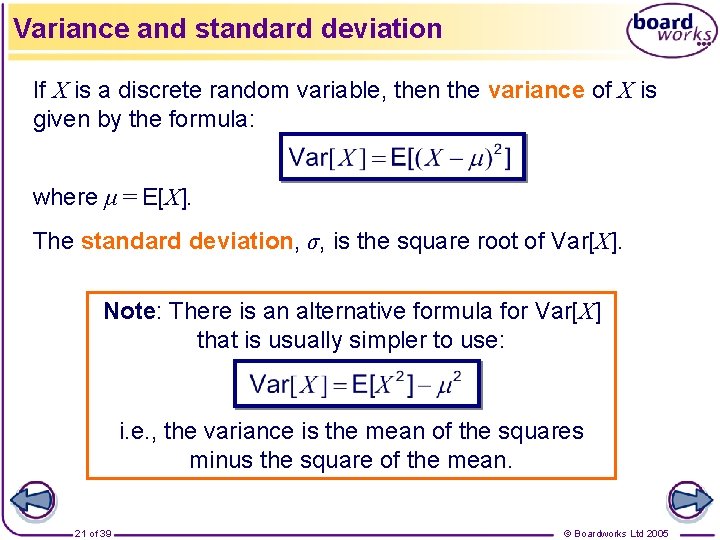
Variance and standard deviation If X is a discrete random variable, then the variance of X is given by the formula: where μ = E[X]. The standard deviation, σ, is the square root of Var[X]. Note: There is an alternative formula for Var[X] that is usually simpler to use: i. e. , the variance is the mean of the squares minus the square of the mean. 21 of 39 © Boardworks Ltd 2005

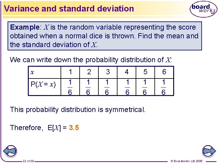
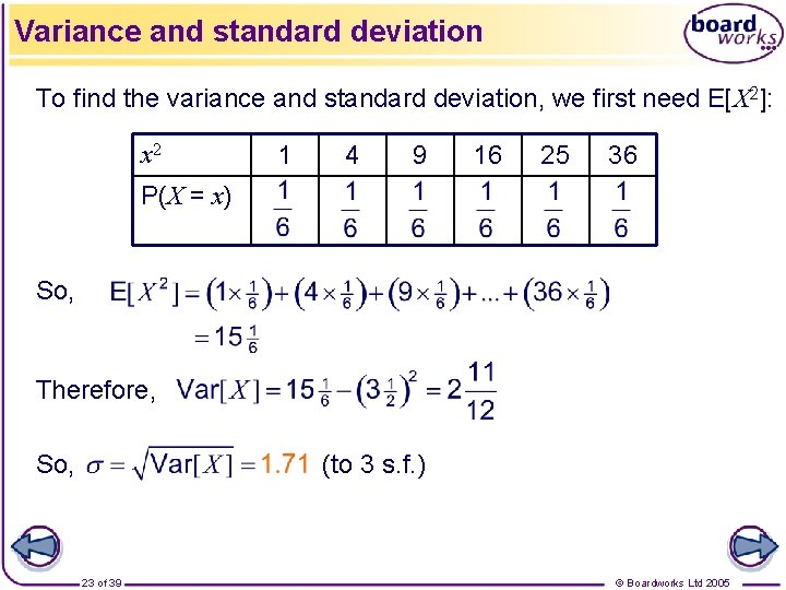
Variance and standard deviation Example: X is the random variable representing the score obtained when a normal dice is thrown. Find the mean and the standard deviation of X. We can write down the probability distribution of X: x 1 2 3 4 5 6 P(X = x) This probability distribution is symmetrical. Therefore, E[X] = 3. 5 22 of 39 © Boardworks Ltd 2005

Variance and standard deviation To find the variance and standard deviation, we first need E[X 2]: x 2 1 4 9 16 25 36 P(X = x) So, Therefore, So, (to 3 s. f. ) 23 of 39 © Boardworks Ltd 2005

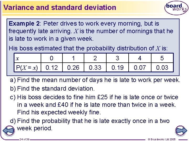
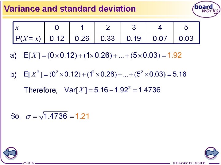
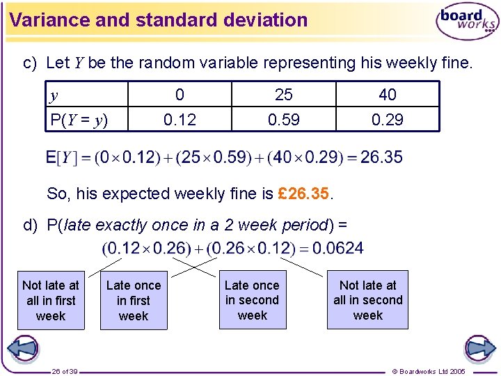
Variance and standard deviation Example 2: Peter drives to work every morning, but is frequently late arriving. X is the number of mornings that he is late to work in a given week. His boss estimated that the probability distribution of X is: x P(X = x) 0 0. 12 1 0. 26 2 0. 33 3 0. 19 4 0. 07 5 0. 03 a) Find the mean number of days he is late to work per week. b) Find the standard deviation. c) His boss decides to fine him £ 25 if he is late once or twice in a week and £ 40 if he is late more than twice in a week. Find his expected weekly fine. d) Find the probability that he is late exactly once in a two week period. 24 of 39 © Boardworks Ltd 2005

Variance and standard deviation x P(X = x) 0 0. 12 1 0. 26 2 0. 33 3 0. 19 4 0. 07 5 0. 03 a) b) Therefore, So, 25 of 39 © Boardworks Ltd 2005

Variance and standard deviation c) Let Y be the random variable representing his weekly fine. y P(Y = y) 0 0. 12 25 0. 59 40 0. 29 So, his expected weekly fine is £ 26. 35. d) P(late exactly once in a 2 week period) = Not late at all in first week 26 of 39 Late once in first week Late once in second week Not late at all in second week © Boardworks Ltd 2005

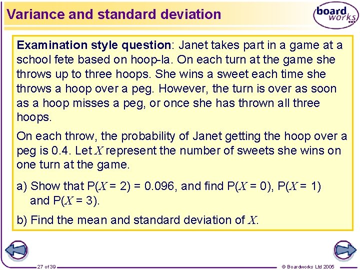
Variance and standard deviation Examination style question: Janet takes part in a game at a school fete based on hoop-la. On each turn at the game she throws up to three hoops. She wins a sweet each time she throws a hoop over a peg. However, the turn is over as soon as a hoop misses a peg, or once she has thrown all three hoops. On each throw, the probability of Janet getting the hoop over a peg is 0. 4. Let X represent the number of sweets she wins on one turn at the game. a) Show that P(X = 2) = 0. 096, and find P(X = 0), P(X = 1) and P(X = 3). b) Find the mean and standard deviation of X. 27 of 39 © Boardworks Ltd 2005

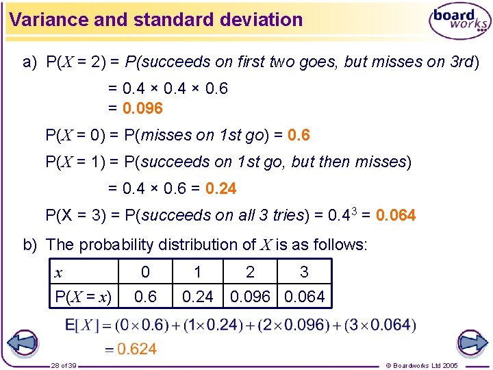
Variance and standard deviation a) P(X = 2) = P(succeeds on first two goes, but misses on 3 rd) = 0. 4 × 0. 6 = 0. 096 P(X = 0) = P(misses on 1 st go) = 0. 6 P(X = 1) = P(succeeds on 1 st go, but then misses) = 0. 4 × 0. 6 = 0. 24 P(X = 3) = P(succeeds on all 3 tries) = 0. 43 = 0. 064 b) The probability distribution of X is as follows: x P(X = x) 28 of 39 0 0. 6 1 2 3 0. 24 0. 096 0. 064 © Boardworks Ltd 2005

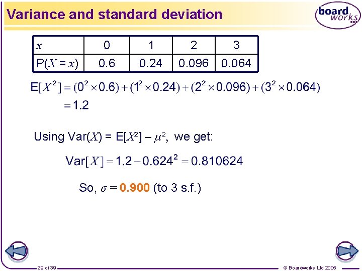
Variance and standard deviation x P(X = x) 0 0. 6 1 0. 24 2 0. 096 3 0. 064 Using Var(X) = E[X²] – μ ², we get: So, σ = 0. 900 (to 3 s. f. ) 29 of 39 © Boardworks Ltd 2005

Discrete uniform distribution Introduction to discrete random variables Contents Cumulative distribution functions Expectation Variance and standard deviation for random variables Discrete uniform distribution Expectation algebra – some key results 30 of 39 © Boardworks Ltd 2005

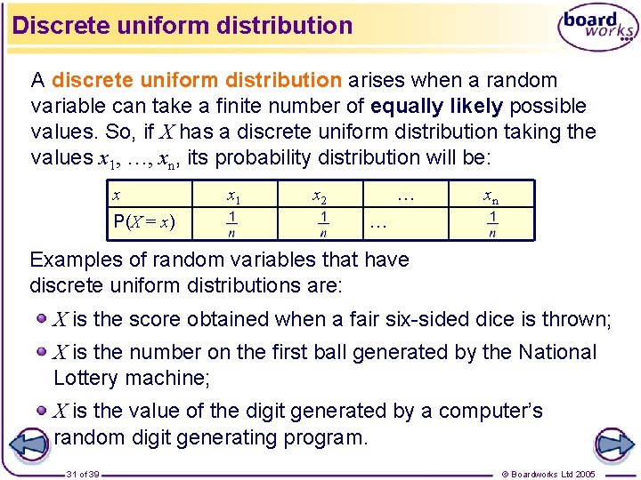
Discrete uniform distribution A discrete uniform distribution arises when a random variable can take a finite number of equally likely possible values. So, if X has a discrete uniform distribution taking the values x 1, …, xn, its probability distribution will be: x P(X = x) x 1 x 2 … xn … Examples of random variables that have discrete uniform distributions are: X is the score obtained when a fair six-sided dice is thrown; X is the number on the first ball generated by the National Lottery machine; X is the value of the digit generated by a computer’s random digit generating program. 31 of 39 © Boardworks Ltd 2005

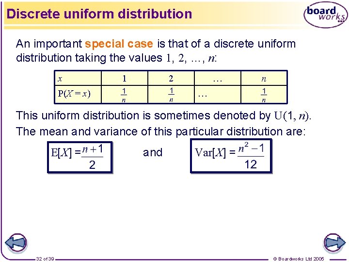
Discrete uniform distribution An important special case is that of a discrete uniform distribution taking the values 1, 2, …, n: x 1 2 P(X = x) … n … This uniform distribution is sometimes denoted by U(1, n). The mean and variance of this particular distribution are: E[X] = 32 of 39 and Var[X] = © Boardworks Ltd 2005

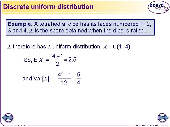
Discrete uniform distribution Example: A tetrahedral dice has its faces numbered 1, 2, 3 and 4. X is the score obtained when the dice is rolled. X therefore has a uniform distribution, X ~ U(1, 4). So, E[X] = and Var[X] = 33 of 39 © Boardworks Ltd 2005

Expectation algebra Introduction to discrete random variables Contents Cumulative distribution functions Expectation Variance and standard deviation for random variables Discrete uniform distribution Expectation algebra – some key results 34 of 39 © Boardworks Ltd 2005

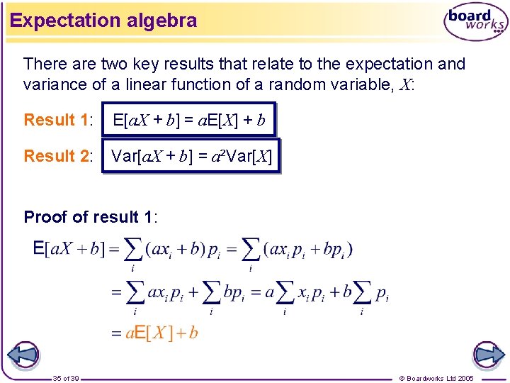
Expectation algebra There are two key results that relate to the expectation and variance of a linear function of a random variable, X: Result 1: E[a. X + b] = a. E[X] + b Result 2: Var[a. X + b] = a²Var[X] Proof of result 1: 35 of 39 © Boardworks Ltd 2005

Expectation algebra Result 2: Var[a. X + b] = a²Var[X] Proof of result 2: Remember: where μ = E[X] 36 of 39 © Boardworks Ltd 2005

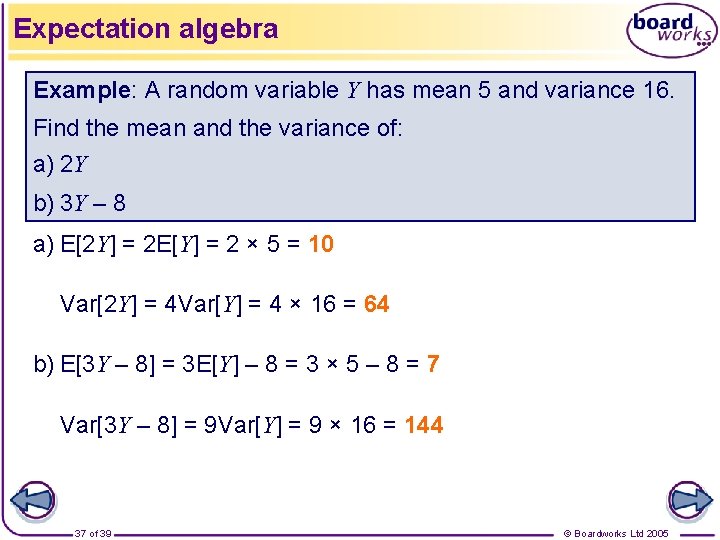
Expectation algebra Example: A random variable Y has mean 5 and variance 16. Find the mean and the variance of: a) 2 Y b) 3 Y – 8 a) E[2 Y] = 2 E[Y] = 2 × 5 = 10 Var[2 Y] = 4 Var[Y] = 4 × 16 = 64 b) E[3 Y – 8] = 3 E[Y] – 8 = 3 × 5 – 8 = 7 Var[3 Y – 8] = 9 Var[Y] = 9 × 16 = 144 37 of 39 © Boardworks Ltd 2005

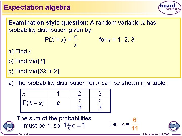
Expectation algebra Examination style question: A random variable X has probability distribution given by: P(X = x) = for x = 1, 2, 3 a) Find c. b) Find Var[X] c) Find Var[6 X + 2]. a) The probability distribution for X can be shown in a table: x P(X = x) 1 c 2 The sum of the probabilities must be 1, so 38 of 39 3 i. e. c = © Boardworks Ltd 2005

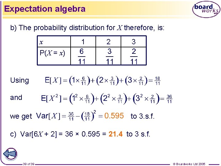
Expectation algebra b) The probability distribution for X therefore, is: x P(X = x) 1 2 3 Using and we get to 3. s. f. c) Var[6 X + 2] = 36 × 0. 595 = 21. 4 to 3 s. f. 39 of 39 © Boardworks Ltd 2005