A Practical Workshop on EXAFS Shell Fitting for

A Practical Workshop on EXAFS Shell Fitting for Environmental Samples Matt Siebecker, Ph. D Delaware Environmental Institute August 17, 2016

Outline for Today’s Workshop • Three hour morning session – – – – Goal for this workshop Purpose of shell fitting How do we do shell fitting EXAFS signal & Fourier Transform EXAFS equation and it’s variables Five variables generally fit by user Knowing when the fit is done • Hamilton test – What parameters to publish? – Example (Ni-foil) • Three hour afternoon session – Small group practice – nickel foil – Small group practice – nickel hydroxide – Small group practice – nickel reacted with pyrophyllite (6 yrs)

Goals for this Workshop • #1 goal is to learn the basics of how to perform shell fitting of EXAFS data using Artemis – Ask questions, promote discussion • Present basic techniques to fit “shells” of a Fourier transformed EXAFS spectrum – Briefly illustrate background subtraction & normalization – Provide a basic “protocol” for getting data loaded and starting a fit • A “crash course” to give you the skills to learn how to fit and provide learning resources – Cannot be learned in one day, or several days – Each system is distinct (crystalline, amorphous, sorption …)

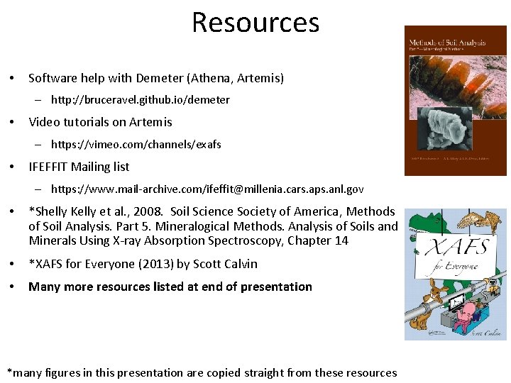
Resources • Software help with Demeter (Athena, Artemis) – http: //bruceravel. github. io/demeter • Video tutorials on Artemis – https: //vimeo. com/channels/exafs • IFEFFIT Mailing list – https: //www. mail-archive. com/ifeffit@millenia. cars. aps. anl. gov • *Shelly Kelly et al. , 2008. Soil Science Society of America, Methods of Soil Analysis. Part 5. Mineralogical Methods. Analysis of Soils and Minerals Using X-ray Absorption Spectroscopy, Chapter 14 • *XAFS for Everyone (2013) by Scott Calvin • Many more resources listed at end of presentation *many figures in this presentation are copied straight from these resources

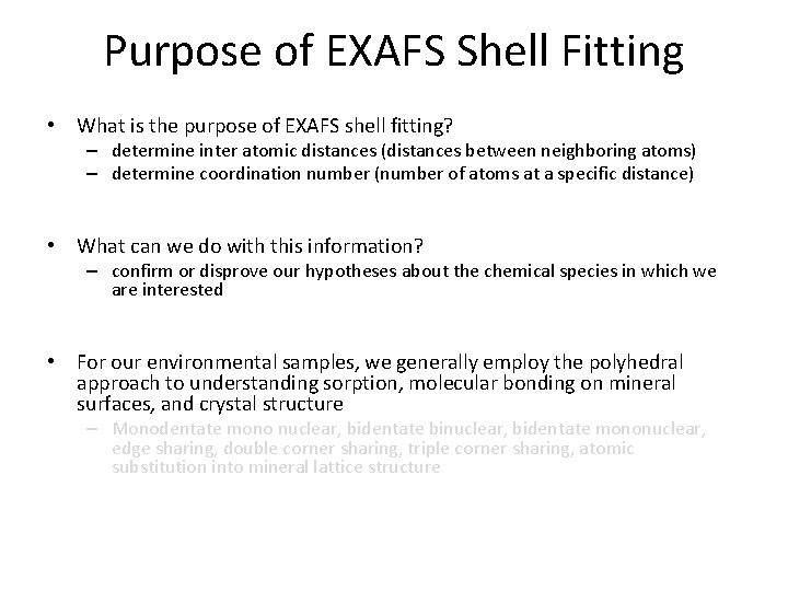
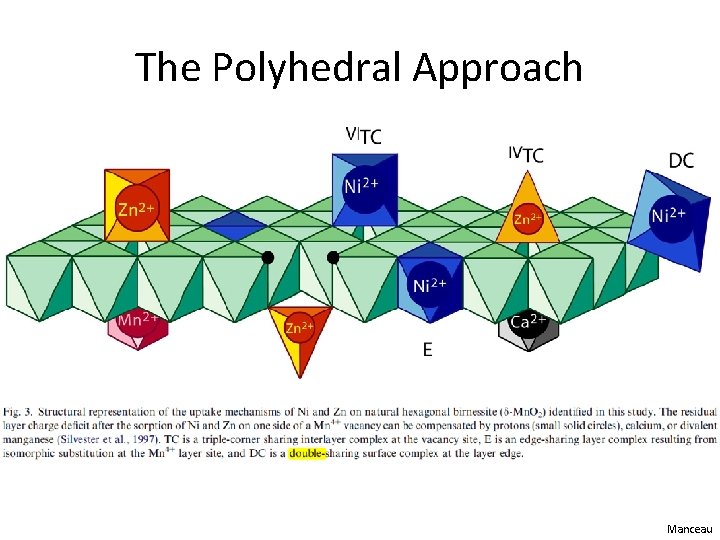
Purpose of EXAFS Shell Fitting • What is the purpose of EXAFS shell fitting? – determine inter atomic distances (distances between neighboring atoms) – determine coordination number (number of atoms at a specific distance) • What can we do with this information? – confirm or disprove our hypotheses about the chemical species in which we are interested • For our environmental samples, we generally employ the polyhedral approach to understanding sorption, molecular bonding on mineral surfaces, and crystal structure – Monodentate mono nuclear, bidentate binuclear, bidentate mononuclear, edge sharing, double corner sharing, triple corner sharing, atomic substitution into mineral lattice structure

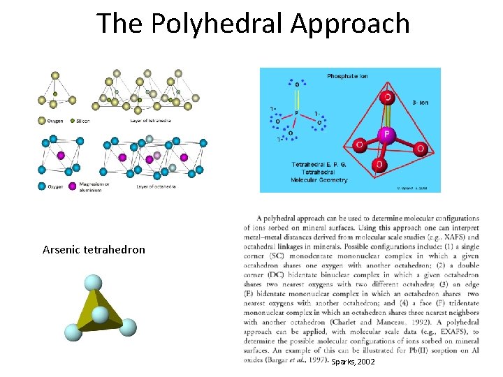
The Polyhedral Approach Arsenic tetrahedron Sparks, 2002

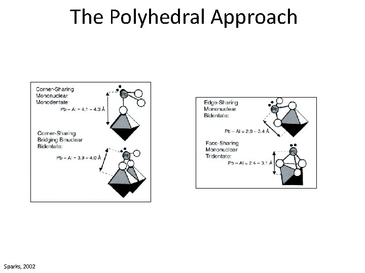
The Polyhedral Approach Sparks, 2002

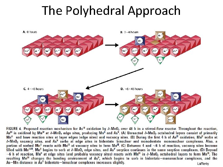
The Polyhedral Approach Lafferty

The Polyhedral Approach Manceau

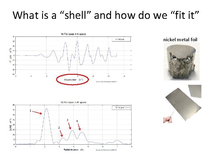
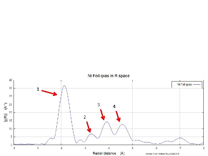
What is a “shell” and how do we “fit it” nickel metal foil

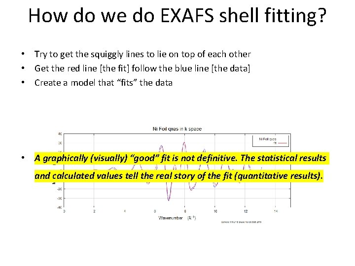
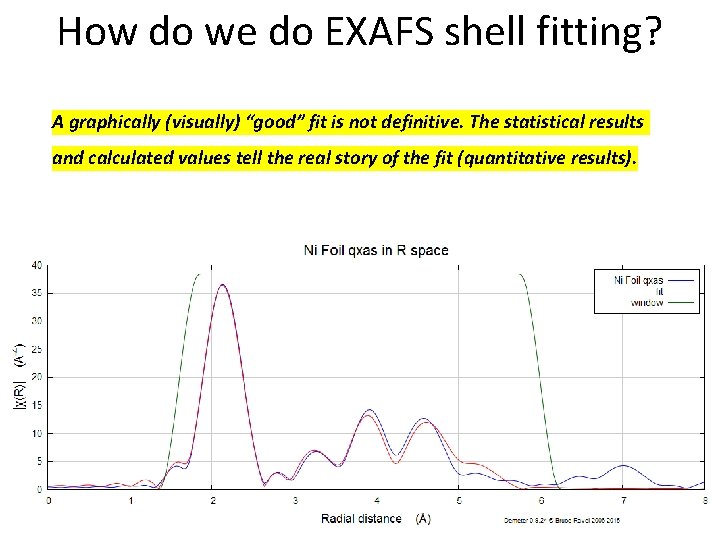
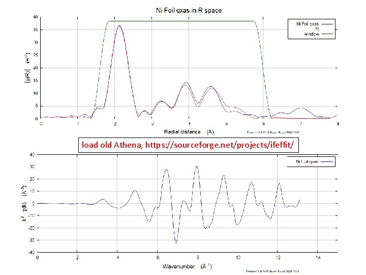
How do we do EXAFS shell fitting? • Try to get the squiggly lines to lie on top of each other • Get the red line [the fit] follow the blue line [the data] • Create a model that “fits” the data • A graphically (visually) “good” fit is not definitive. The statistical results and calculated values tell the real story of the fit (quantitative results).

How do we do EXAFS shell fitting? A graphically (visually) “good” fit is not definitive. The statistical results and calculated values tell the real story of the fit (quantitative results).

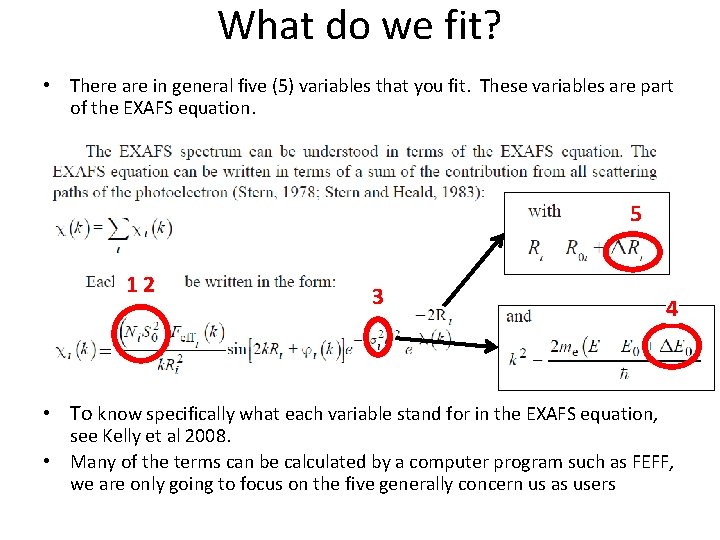
What statistical results and calculated values? • There are in general five (5) variables that you fit. These variables are part of the EXAFS equation. • The EXAFS equation describes the features seen in EXAFS data (e. g. , amplitude and frequency of oscillations) – to determine interatomic distances and coordination number we fit five variables that are part of the EXAFS equation. • Create the best fit possible with the least number of fitted variables – “BEST FIT” = physically realistic values with lowest amount of misfit using least amount of fitted variables – R-factor, “chi square” (χ2), “reduced chi square” (χ2 v) – “chi” is pronounced “kahy” – Using constraints based on prior knowledge about the sample • Crystal structure, predicted interatomic distances, disorder (amorphous vs, crystalline)

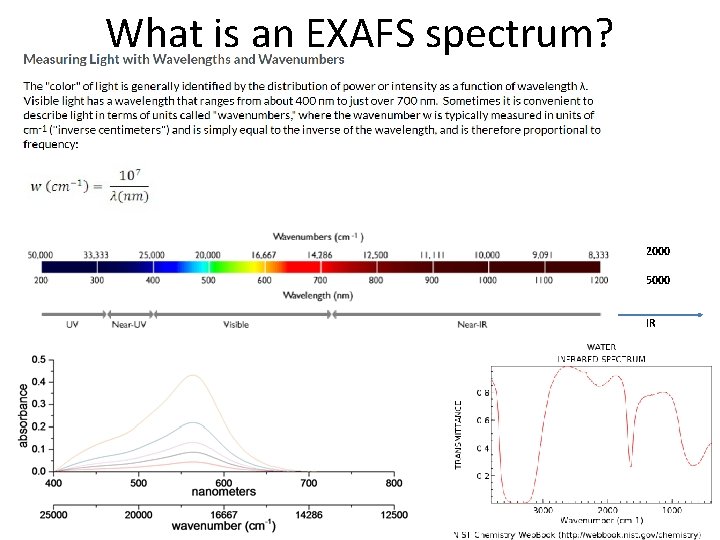
What is an EXAFS spectrum? 2000 5000 IR

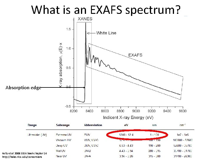
What is an EXAFS spectrum? Absorption edge Kelly et al 2008 SSSA book chapter 14 http: //halas. rice. edu/conversions

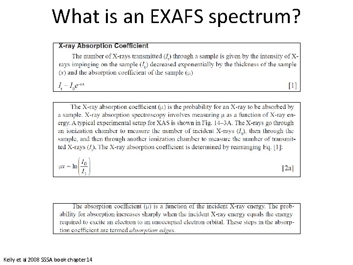
What is an EXAFS spectrum? Kelly et al 2008 SSSA book chapter 14

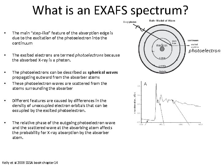
What is an EXAFS spectrum? • The main “step-like” feature of the absorption edge is due to the excitation of the photoelectron into the continuum • The excited electrons are termed photoelectrons because the absorbed X-ray is a photon. • The photoelectrons can be described as spherical waves propagating outward from the absorber atoms These photoelectron waves are scattered from the atoms surrounding the absorber • • Different features are caused by differences in the density of unoccupied electron orbitals that can be occupied by the excited photoelectron. • The relative phase of the outgoing photoelectron wave and the scattered wave at the absorbing atom affects the probability for X-ray absorption by the absorber atom. Kelly et al 2008 SSSA book chapter 14 photoelectron

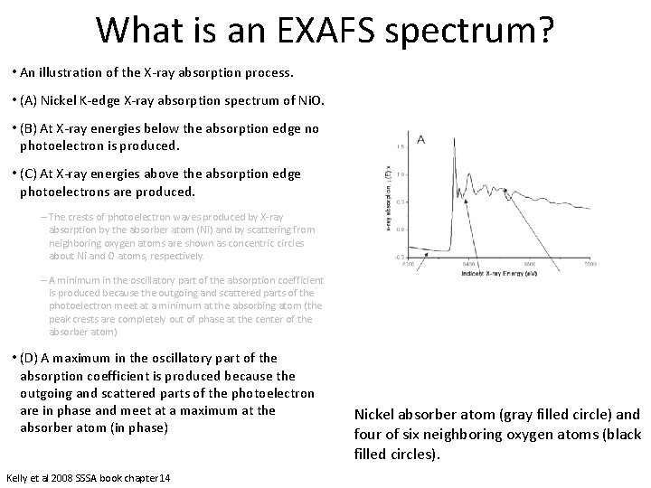
What is an EXAFS spectrum? • An illustration of the X-ray absorption process. • (A) Nickel K-edge X-ray absorption spectrum of Ni. O. • (B) At X-ray energies below the absorption edge no photoelectron is produced. • (C) At X-ray energies above the absorption edge photoelectrons are produced. – The crests of photoelectron waves produced by X-ray absorption by the absorber atom (Ni) and by scattering from neighboring oxygen atoms are shown as concentric circles about Ni and O atoms, respectively. – A minimum in the oscillatory part of the absorption coefficient is produced because the outgoing and scattered parts of the photoelectron meet at a minimum at the absorbing atom (the peak crests are completely out of phase at the center of the absorber atom) • (D) A maximum in the oscillatory part of the absorption coefficient is produced because the outgoing and scattered parts of the photoelectron are in phase and meet at a maximum at the absorber atom (in phase) Kelly et al 2008 SSSA book chapter 14 Nickel absorber atom (gray filled circle) and four of six neighboring oxygen atoms (black filled circles).

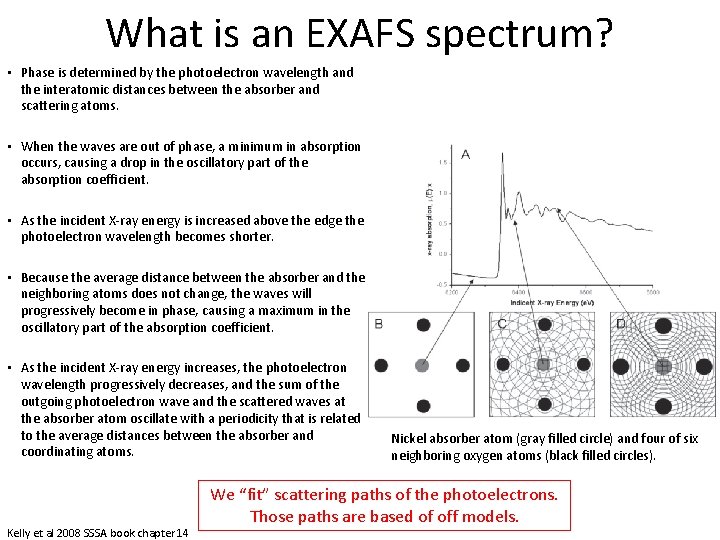
What is an EXAFS spectrum? • Phase is determined by the photoelectron wavelength and the interatomic distances between the absorber and scattering atoms. • When the waves are out of phase, a minimum in absorption occurs, causing a drop in the oscillatory part of the absorption coefficient. • As the incident X-ray energy is increased above the edge the photoelectron wavelength becomes shorter. • Because the average distance between the absorber and the neighboring atoms does not change, the waves will progressively become in phase, causing a maximum in the oscillatory part of the absorption coefficient. • As the incident X-ray energy increases, the photoelectron wavelength progressively decreases, and the sum of the outgoing photoelectron wave and the scattered waves at the absorber atom oscillate with a periodicity that is related to the average distances between the absorber and coordinating atoms. Kelly et al 2008 SSSA book chapter 14 Nickel absorber atom (gray filled circle) and four of six neighboring oxygen atoms (black filled circles). We “fit” scattering paths of the photoelectrons. Those paths are based of off models.

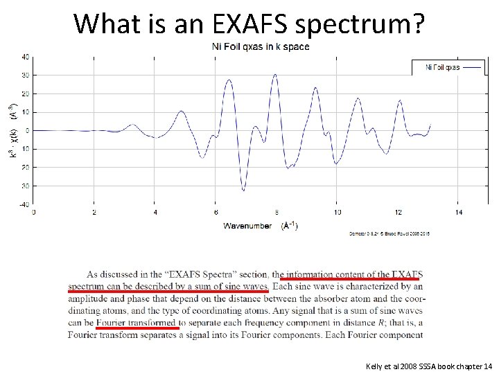
What is an EXAFS spectrum? Kelly et al 2008 SSSA book chapter 14

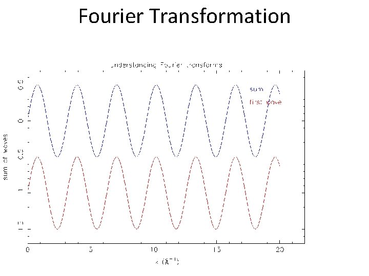
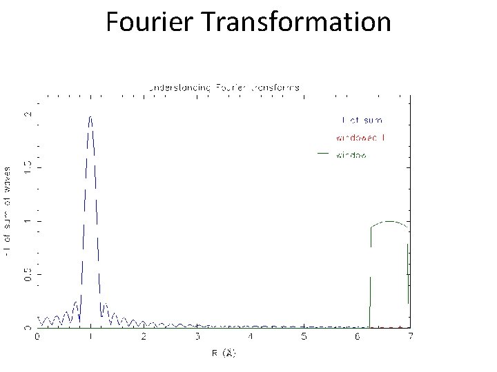
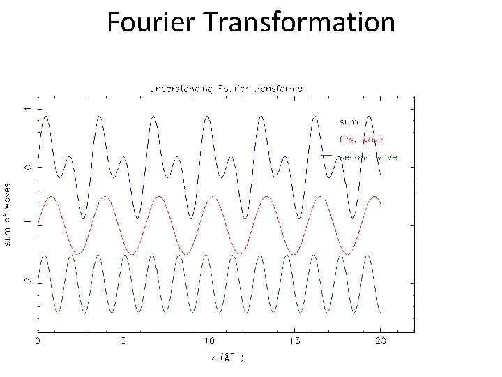
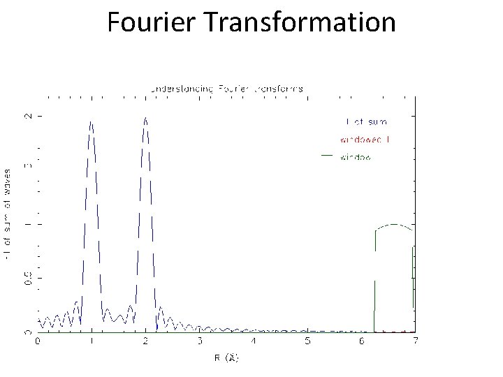
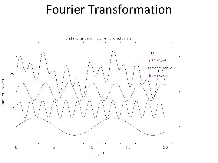
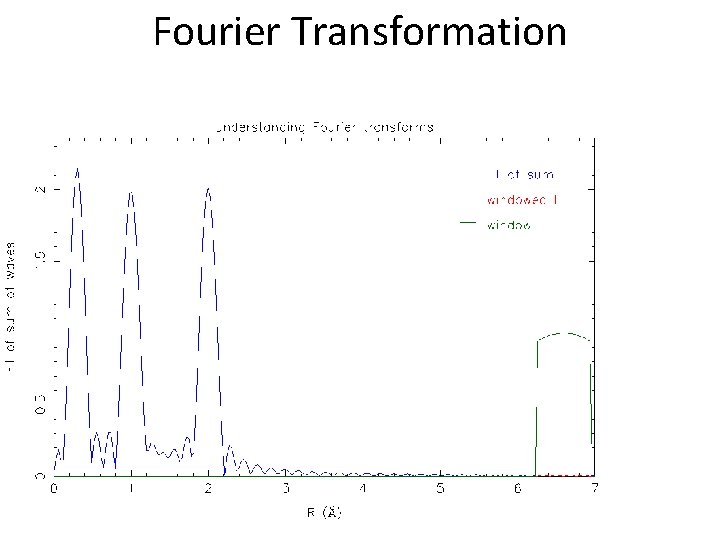
Fourier Transformation

Fourier Transformation

Fourier Transformation

Fourier Transformation

Fourier Transformation

Fourier Transformation

Fourier Transformation load old Athena, https: //sourceforge. net/projects/ifeffit/

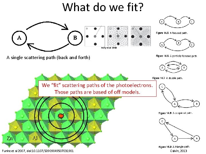
What do we fit? Kelly et al 2008 A single scattering path (back and forth) We “fit” scattering paths of the photoelectrons. Those paths are based of off models. Funke et al 2007, doi: 10. 1107/S 0909049507031901 Calvin, 2013

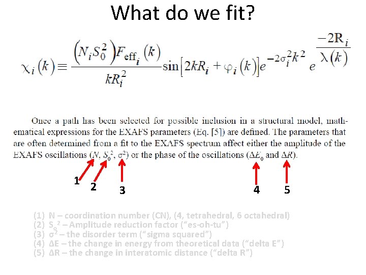
What do we fit? • There are in general five (5) variables that you fit. These variables are part of the EXAFS equation. 5 12 3 • To know specifically what each variable stand for in the EXAFS equation, 4 see Kelly et al 2008. • Many of the terms can be calculated by a computer program such as FEFF, we are only going to focus on the five generally concern us as users

What do we fit? 1 2 (1) (2) (3) (4) (5) 3 4 5 N – coordination number (CN), (4, tetrahedral, 6 octahedral) So 2 – Amplitude reduction factor (“es-oh-tu”) σ2 – the disorder term (“sigma squared”) ΔE – the change in energy from theoretical data (“delta E”) ΔR – the change in interatomic distance (“delta R”)

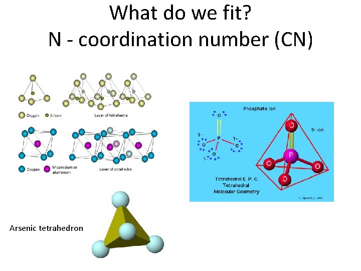
What do we fit? N - coordination number (CN) • Degeneracy (the number of equal path lengths) – For tetrahedrally coordinated atoms (arsenate, arsenite, phosphate), CN=4 – For octahedrally coordinated atoms (hydroxide sheets, many aqueous metal ions), CN=6 • Typical values – never negative, generally less than 8 for oxides for single scattering • When fitting a “standard” this value can be constrained to equal the CN of the model to determine So 2 • Generally for the first shell, we have a good idea if it is 4 or close to 6 (tetrahedral or octahedral) – For the second shell, It is guessed when fitting an unknown CN (e. g. , sorption sample or precipitate)

What do we fit? N - coordination number (CN) Arsenic tetrahedron

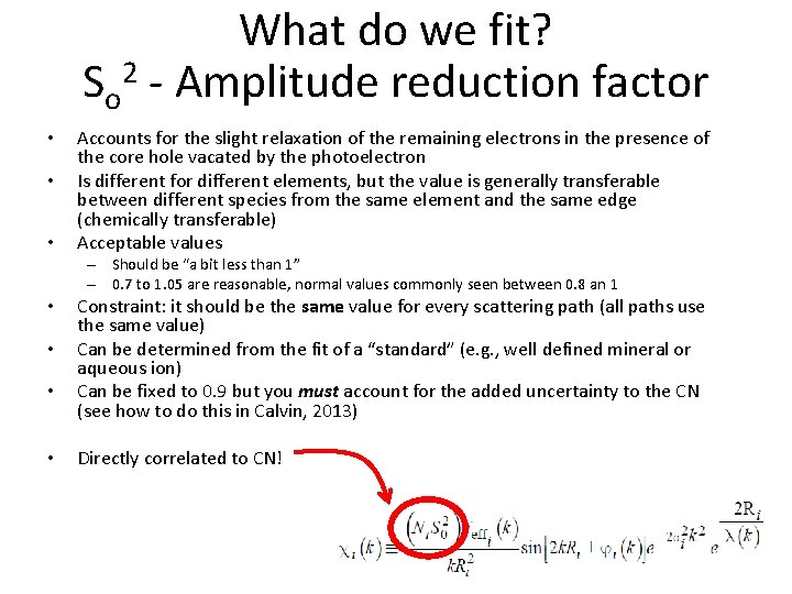
What do we fit? 2 So - Amplitude reduction factor • • • Accounts for the slight relaxation of the remaining electrons in the presence of the core hole vacated by the photoelectron Is different for different elements, but the value is generally transferable between different species from the same element and the same edge (chemically transferable) Acceptable values – Should be “a bit less than 1” – 0. 7 to 1. 05 are reasonable, normal values commonly seen between 0. 8 an 1 • • Constraint: it should be the same value for every scattering path (all paths use the same value) Can be determined from the fit of a “standard” (e. g. , well defined mineral or aqueous ion) Can be fixed to 0. 9 but you must account for the added uncertainty to the CN (see how to do this in Calvin, 2013) Directly correlated to CN!

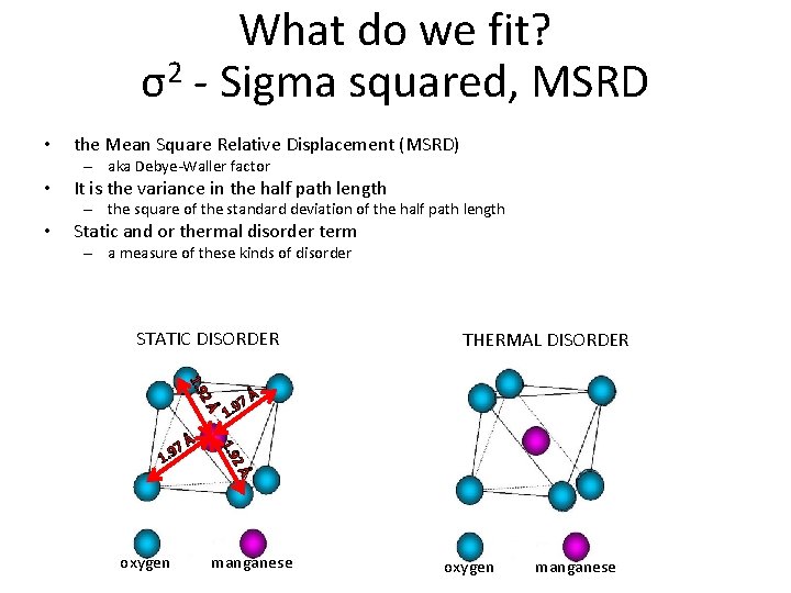
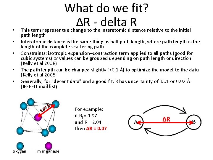
What do we fit? 2 σ - Sigma squared, MSRD • the Mean Square Relative Displacement (MSRD) – aka Debye-Waller factor • It is the variance in the half path length – the square of the standard deviation of the half path length • Static and or thermal disorder term – a measure of these kinds of disorder STATIC DISORDER 2Å 1. 9 2Å oxygen Å Å 1. 9 7 1. 9 THERMAL DISORDER manganese oxygen manganese

What do we fit? 2 σ - Sigma squared, MSRD • In general, the values for σ2 become bigger with increasing bond length or shell number (Kelly et al. , 2008) – E. g. , 0. 006 for first shell, 0. 01 for second shell • Typical values: 0. 002 to 0. 03 Å2, if any larger, the path is so disordered that it is contributing little to the fit which can be a sign the model is wrong in some way (Calvin, 2013) • There are many, many ways to constrain this variable: – Use one value “constrain” for atoms of similar type (Z) and similar distance – Constrain values for atoms overlapping in their error bars – Use one value for the first shell and one value for the second shell – See Calvin, 2013 for more discussion

What do we fit? ΔE – “delta E” (E 0, “Enot”) • This term relates to a change in the photoelectron energy and is used to align the energy scale of theoretical spectrum to match the measured spectrum (Kelly et al. , 2008) – https: //www. researchgate. net/publication/237626147_EXAFS_Energ y_Shift_and_Structural_Parameters • In general, these shifts should be less than 2 to 3 e. V – See “Aligning Energy Scales of Experimental and Theoretical Spectra” in Kelly et al. , 2008 for adjust for shifts larger than this – Generally, for "decent data" and a good fit E 0 has uncertainty of 0. 5 to 1. 0 e. V (IFEFFIT mail list) • E 0 should always be on or near the rising portion of the edge, never on the smooth pre-edge or in the EXAFS region (Calvin, 2013) • Constraint: Use one ΔE for all scattering paths

• • • What do we fit? ΔR - delta R This term represents a change to the interatomic distance relative to the initial path length Interatomic distance is the same thing as half path length, where path length is the length of the complete scattering path Constraints: isotropic expansion–contraction term applied to all paths (good for cubic systems) or values can be grouped depending on path length or direction (Kelly et al 2008) The path length can be changed slightly (<0. 1 Å) to optimize the model to the data (Kelly et al 2008 Generally, for "decent data" and a good fit, R has uncertainty of 0. 01 or 0. 02 Å (IFEFFIT mail list) 7 1. 9 oxygen Å manganese For example: if Ri = 1. 97 and R = 2. 04 then ΔR = 0. 07 ΔR

Constraints - Why would constraining your fit be a good idea? • A constrained fit shows that your model and data are in good agreement (i. e. , the data are what you thought they were) • A constrained fit reduces the number of fitted variables, which supports your argument that your data are similar to the model you’ve chosen • A constrained fit decreases your reduced chi square value (a statistical parameter used to measure goodness-of-fit) • A constrained fit can help keep variables in a physically realistic range of results – sometimes variables, when given too much freedom, will change too much and move out of acceptable ranges in order to improve the fit. By constraining them, you keep them where they should be while maintaining reasonable fitting parameters

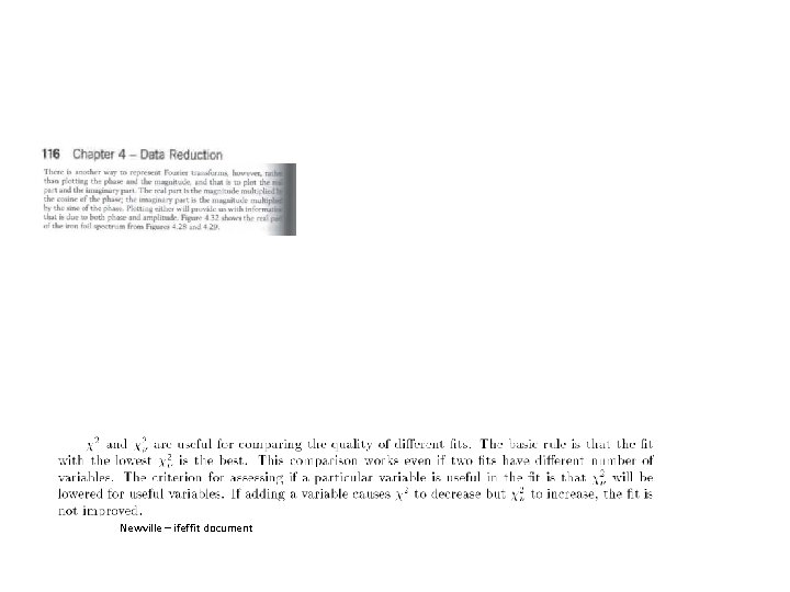
Fit statistics – How good is the fit? • Statistical parameters (the standard goodness-of fit parameters) include: – the number of independent points, Nidp – the number of variables, Nvar – – • must be less than Nidp “chi square” (χ2) “reduced chi square” (χ2 v) R-factor All these values are calculated by the software (except Nvar) • The isolated EXAFS signal is denoted as χ(k) and should not be confused with the goodness-of-fit parameter χ2 • Changes in the goodness-of-fit parameter χ2 v are used to compare fits with different number of variables (Nvar) • The R factor is a major fit parameter that needs to be included in the published table

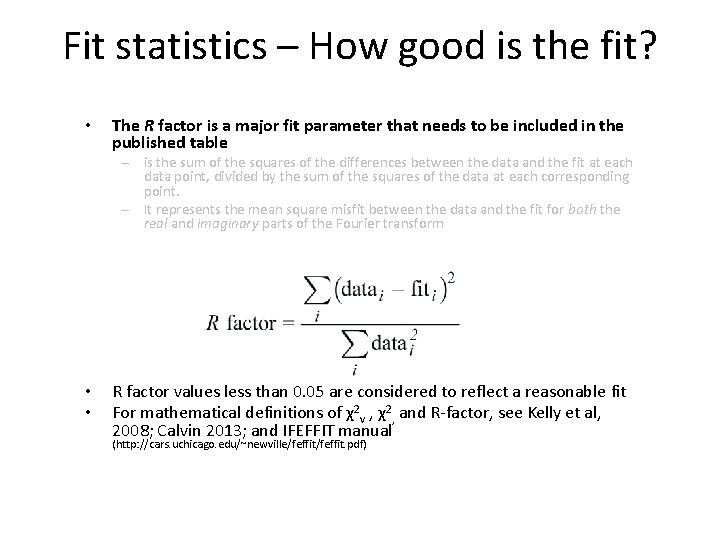
Fit statistics – How good is the fit? • The R factor is a major fit parameter that needs to be included in the published table – is the sum of the squares of the differences between the data and the fit at each data point, divided by the sum of the squares of the data at each corresponding point. – It represents the mean square misfit between the data and the fit for both the real and imaginary parts of the Fourier transform • • R factor values less than 0. 05 are considered to reflect a reasonable fit For mathematical definitions of χ2 v , χ2, and R-factor, see Kelly et al, 2008; Calvin 2013; and IFEFFIT manual (http: //cars. uchicago. edu/~newville/feffit. pdf)

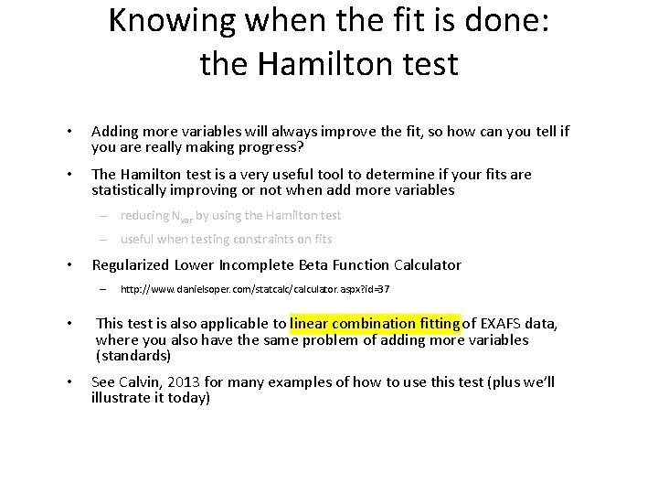
Knowing when the fit is done: the Hamilton test • Adding more variables will always improve the fit, so how can you tell if you are really making progress? • The Hamilton test is a very useful tool to determine if your fits are statistically improving or not when add more variables – reducing Nvar by using the Hamilton test – useful when testing constraints on fits • Regularized Lower Incomplete Beta Function Calculator – http: //www. danielsoper. com/statcalc/calculator. aspx? id=37 • This test is also applicable to linear combination fitting of EXAFS data, where you also have the same problem of adding more variables (standards) • See Calvin, 2013 for many examples of how to use this test (plus we’ll illustrate it today)

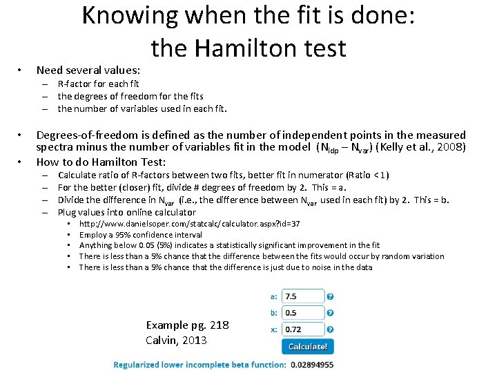
• Knowing when the fit is done: the Hamilton test Need several values: – R-factor for each fit – the degrees of freedom for the fits – the number of variables used in each fit. • • Degrees-of-freedom is defined as the number of independent points in the measured spectra minus the number of variables fit in the model (Nidp – Nvar) (Kelly et al. , 2008) How to do Hamilton Test: – – Calculate ratio of R-factors between two fits, better fit in numerator (Ratio < 1) For the better (closer) fit, divide # degrees of freedom by 2. This = a. Divide the difference in Nvar (i. e. , the difference between Nvar used in each fit) by 2. This = b. Plug values into online calculator • • • http: //www. danielsoper. com/statcalc/calculator. aspx? id=37 Employ a 95% confidence interval Anything below 0. 05 (5%) indicates a statistically significant improvement in the fit There is less than a 5% chance that the difference between the fits would occur by random variation There is less than a 5% chance that the difference is just due to noise in the data Example pg. 218 Calvin, 2013

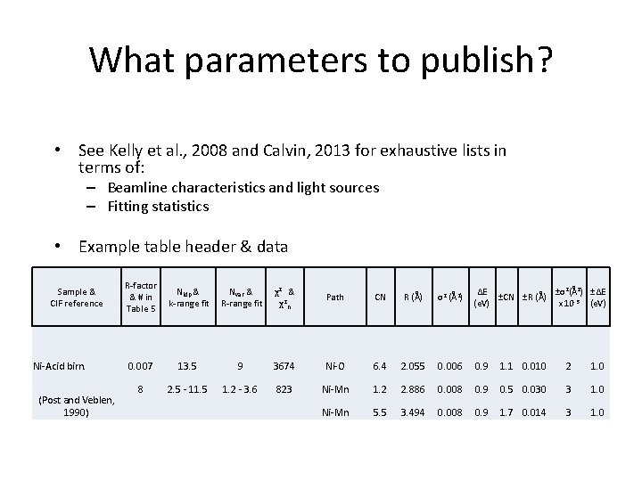
What parameters to publish? • See Kelly et al. , 2008 and Calvin, 2013 for exhaustive lists in terms of: – Beamline characteristics and light sources – Fitting statistics • Example table header & data Sample & CIF reference Ni-Acid birn. (Post and Veblen, 1990) R-factor Nidp & Nvar & & # in k-range fit R-range fit Table 5 χ2 & χ2 n Path CN R (Å) σ2 (Å2) ΔE ±σ2(Å2) ±ΔE ±CN ±R (Å) (e. V) x 10 -3 (e. V) 0. 007 13. 5 9 3674 Ni-O 6. 4 2. 055 0. 006 0. 9 1. 1 0. 010 2 1. 0 8 2. 5 - 11. 5 1. 2 - 3. 6 823 Ni-Mn 1. 2 2. 886 0. 008 0. 9 0. 5 0. 030 3 1. 0 Ni-Mn 5. 5 3. 494 0. 008 0. 9 1. 7 0. 014 3 1. 0

Resources • Software help – http: //bruceravel. github. io/demeter/ • Video tutorials – https: //vimeo. com/channels/exafs • Mailing list – https: //www. mailarchive. com/ifeffit@millenia. cars. aps. anl. gov/ • Hamilton Test calculator – http: //www. danielsoper. com/statcalc/calcula tor. aspx? id=37

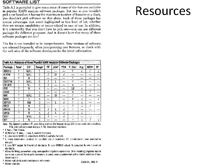
Resources Calvin, 2013

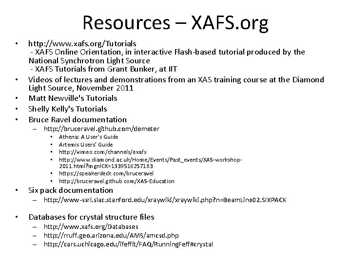
Resources – XAFS. org • • • http: //www. xafs. org/Tutorials - XAFS Online Orientation, in interactive Flash-based tutorial produced by the National Synchrotron Light Source - XAFS Tutorials from Grant Bunker, at IIT Videos of lectures and demonstrations from an XAS training course at the Diamond Light Source, November 2011 Matt Newville's Tutorials Shelly Kelly's Tutorials Bruce Ravel documentation – http: //bruceravel. github. com/demeter • • Athena: A User's Guide Artemis Users' Guide http: //vimeo. com/channels/exafs http: //www. diamond. ac. uk/Home/Events/Past_events/XAS-workshop 2011. html? mgnl. CK=1339516257183 https: //speakerdeck. com/bruceravel http: //bruceravel. github. com/XAS-Education Six pack documentation – http: //www-ssrl. slac. stanford. edu/xraywiki. php? n=Beam. Line 02. SIXPACK • Databases for crystal structure files – http: //www. xafs. org/Databases – http: //rruff. geo. arizona. edu/AMS/amcsd. php – http: //cars. uchicago. edu/ifeffit/FAQ/Running. Feff#crystal

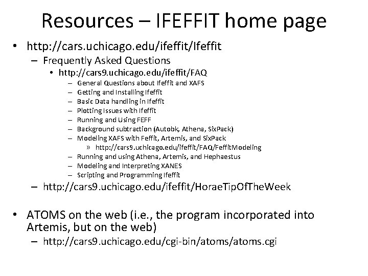
Resources – IFEFFIT home page • http: //cars. uchicago. edu/ifeffit/Ifeffit – Frequently Asked Questions • http: //cars 9. uchicago. edu/ifeffit/FAQ General Questions about Ifeffit and XAFS Getting and Installing Ifeffit Basic Data handling in Ifeffit Plotting Issues with Ifeffit Running and Using FEFF Background subtraction (Autobk, Athena, Six. Pack) Modeling XAFS with Feffit, Artemis, and Six. Pack » http: //cars 9. uchicago. edu/ifeffit/FAQ/Feffit. Modeling – Running and using Athena, Artemis, and Hephaestus – Modeling and Interpreting XANES – Scripting and Programming Ifeffit – – – – http: //cars 9. uchicago. edu/ifeffit/Horae. Tip. Of. The. Week • ATOMS on the web (i. e. , the program incorporated into Artemis, but on the web) – http: //cars 9. uchicago. edu/cgi-bin/atoms. cgi

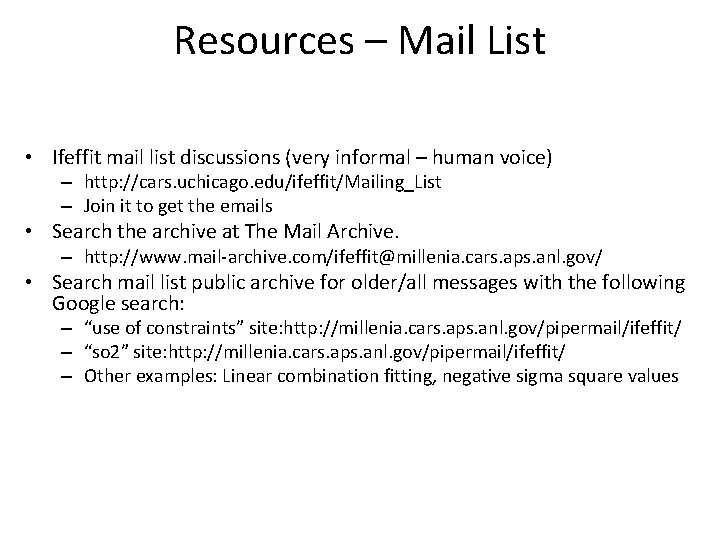
Resources – Mail List • Ifeffit mail list discussions (very informal – human voice) – http: //cars. uchicago. edu/ifeffit/Mailing_List – Join it to get the emails • Search the archive at The Mail Archive. – http: //www. mail-archive. com/ifeffit@millenia. cars. aps. anl. gov/ • Search mail list public archive for older/all messages with the following Google search: – “use of constraints” site: http: //millenia. cars. aps. anl. gov/pipermail/ifeffit/ – “so 2” site: http: //millenia. cars. aps. anl. gov/pipermail/ifeffit/ – Other examples: Linear combination fitting, negative sigma square values

Resources – Mail List • Fitting procedure – http: //www. mailarchive. com/ifeffit@millenia. cars. aps. anl. gov/msg 01694. html • Coordination Number – http: //millenia. cars. aps. anl. gov/pipermail/ifeffit/2002 October/000151. html – http: //www. mailarchive. com/ifeffit@millenia. cars. aps. anl. gov/msg 03435. html • Guide Lines for acceptable fitting parameter values – http: //www. mailarchive. com/ifeffit@millenia. cars. aps. anl. gov/msg 01861. html • The use of constraints & restraints in fitting, use of dopants*, other good techniques – http: //millenia. cars. aps. anl. gov/pipermail/ifeffit/2010 -May/009446. html – http: //cars 9. uchicago. edu/feffusers/msg 00047. html • * - very useful knowledge when you need to substitute atoms into/out of feff. inp files – most of you will need to do this at some point

Resources – book chapters & papers • ***Kelly, S. D. , Hesterberg, D. and Ravel, B. (2008). Analysis of soils and minerals using Xray absorption spectroscopy. Methods of soil analysis, Part 5 -Mineralogical methods. Ulery, A. L. and Drees, L. R. Madison, WI, USA, Soil Science Society of America: 367 -463. • Quantitative speciation of heavy metals in soils and sediments by synchrotron X-ray techniques. Author(s): Manceau, A; Marcus, MA; Tamura, N Book Editor(s): Fenter, PA; Rivers, ML; Sturchio, NC; et al. Source: APPLICATIONS OF SYNCHROTRON RADIATION IN LOW-TEMPERATURE GEOCHEMISTRY AND ENVIRONMENTAL SCIENCES Book Series: Reviews in Mineralogy & Geochemistry Volume: 49 Pages: 341 -428 DOI: 10. 2138/gsrmg. 49. 1. 341 Published: 2002 • Fendorf, S. E. , and D. L. Sparks. 1996. X-ray absorption fine structure spectroscopy. In Methods of Soil Analysis: Chemical Methods. J. M. Bigham (Ed), ASA, Madison, WI. . : p. 377 -416. • J. Am. Chem. SOC. 1994, 116, 2938 -2949 Extended X-ray Absorption Fine Structure (EXAFS) Analysis of Disorder and Multiple-Scattering in Complex Crystalline Solids P. A. O'Day. J. Rehr, i S. I. Zabinsky, t and C. E. Brown, Jr.

Resources – book chapters • An overview of synchrotron radiation applications to low temperature geochemistry and environmental science Author(s): Brown, GE; Sturchio, NC Book Editor(s): Fenter, PA; Rivers, ML; Sturchio, NC; et al. Source: APPLICATIONS OF SYNCHROTRON RADIATION IN LOWTEMPERATURE GEOCHEMISTRY AND ENVIRONMENTAL SCIENCES Book Series: Reviews in Mineralogy & Geochemistry Volume: 49 Pages: 1 -115 DOI: 10. 2138/gsrmg. 49. 1. 1 Published: 2002 • Sorption of trace elements on mineral surfaces: Modern perspectives from spectroscopic studies, and comments on sorption in the marine environment Author(s): Brown, GE; Parks, GA Source: INTERNATIONAL GEOLOGY REVIEW Volume: 43 Issue: 11 Pages: 963 -1073 Published: NOV 2001 • Molecular environmental geochemistry. Author(s): O'Day, PA Source: REVIEWS OF GEOPHYSICS Volume: 37 Issue: 2 Pages: 249 -274 DOI: 10. 1029/1998 RG 900003 Published: MAY 1999 • Mineral surfaces and bioavailability of heavy metals: A molecular-scale perspective Author(s): Brown, GE; Foster, AL; Ostergren, JD Source: PROCEEDINGS OF THE NATIONAL ACADEMY OF SCIENCES OF THE UNITED STATES OF AMERICA Volume: 96 Issue: 7 Pages: 3388 -3395 DOI: 10. 1073/pnas. 96. 7. 3388 Published: MAR 30 1999 • Metal oxide surfaces and their interactions with aqueous solutions and microbial organisms Author(s): Brown, GE; Henrich, VE; Casey, WH; et al. Source: CHEMICAL REVIEWS Volume: 99 Issue: 1 Pages: 77 -174 DOI: 10. 1021/cr 980011 z

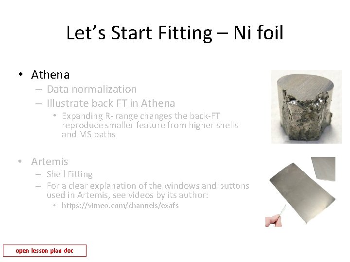
Let’s Start Fitting – Ni foil • Athena – Data normalization – Illustrate back FT in Athena • Expanding R- range changes the back-FT reproduce smaller feature from higher shells and MS paths • Artemis – Shell Fitting – For a clear explanation of the windows and buttons used in Artemis, see videos by its author: • https: //vimeo. com/channels/exafs open lesson plan doc

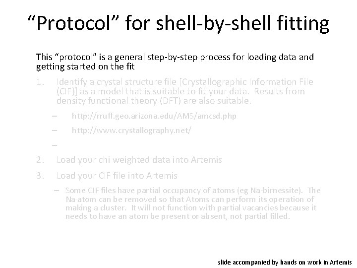
“Protocol” for shell-by-shell fitting This “protocol” is a general step-by-step process for loading data and getting started on the fit 1. Identify a crystal structure file [Crystallographic Information File (CIF)] as a model that is suitable to fit your data. Results from density functional theory (DFT) are also suitable. – http: //rruff. geo. arizona. edu/AMS/amcsd. php – http: //www. crystallography. net/ – 2. Load your chi weighted data into Artemis 3. Load your CIF file into Artemis – Some CIF files have partial occupancy of atoms (eg Na-birnessite). The Na atom can be removed so that Atoms can perform its operation of making a cluster. It will not function with partial vacancies because it needs to have an atom be present or absent, not partial filled. slide accompanied by hands on work in Artemis

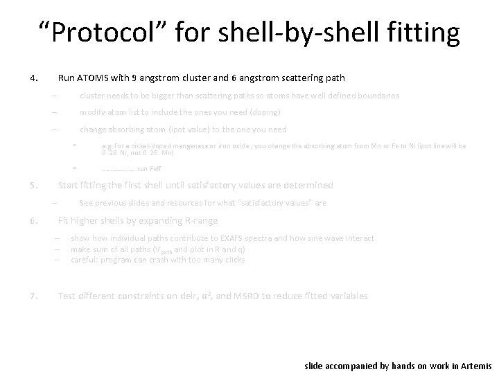
“Protocol” for shell-by-shell fitting 4. Run ATOMS with 9 angstrom cluster and 6 angstrom scattering path – cluster needs to be bigger than scattering paths so atoms have well defined boundaries – modify atom list to include the ones you need (doping) – change absorbing atom (ipot value) to the one you need 5. • ………………. . run Feff See previous slides and resources for what “satisfactory values” are Fit higher shells by expanding R-range – – – 7. e. g. for a nickel-doped manganese or iron oxide , you change the absorbing atom from Mn or Fe to Ni (ipot line will be 0 28 Ni, not 0 25 Mn) Start fitting the first shell until satisfactory values are determined – 6. • show individual paths contribute to EXAFS spectra and how sine wave interact make sum of all paths (V path and plot in R and q) careful: program can crash with too many clicks Test different constraints on delr, σ2, and MSRD to reduce fitted variables slide accompanied by hands on work in Artemis

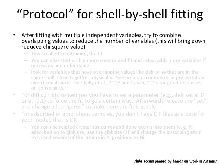
“Protocol” for shell-by-shell fitting • After fitting with multiple independent variables, try to combine overlapping values to reduce the number of variables (this will bring down reduced chi square value) – This is called constraining the fit – You can also start with a more constrained fit and relax (add) more variables if necessary and defendable – look for variables that have overlapping values like delr or ss that are in the same shell, close together physically. See previous comments in presentation about constraints. See Kelly et al. , 2008 and Calvin, 2013 for good recourses on constraints. • For difficult fits sometimes you have to set a parameter (e. g. , delr set at 0 or at -0. 1) to force the fit to go a certain way. Afterwards release the “set” and change all to “guess” to make sure the fit is stable • For adsorbed or amorphous samples, you don’t have CIF files as a base for your model, that is OK – You can use related crystal structures and dope atoms into them (e. g. , Ni adsorbed on to gibbsite, use the gibbsite CIF and change the absorbing atom to Ni and several of the atoms in Al positions to Ni. slide accompanied by hands on work in Artemis

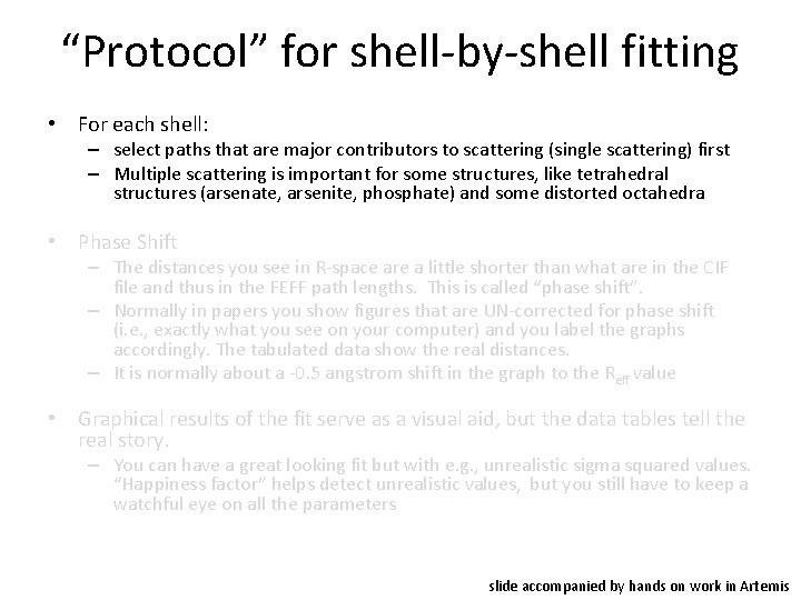
“Protocol” for shell-by-shell fitting • For each shell: – select paths that are major contributors to scattering (single scattering) first – Multiple scattering is important for some structures, like tetrahedral structures (arsenate, arsenite, phosphate) and some distorted octahedra • Phase Shift – The distances you see in R-space are a little shorter than what are in the CIF file and thus in the FEFF path lengths. This is called “phase shift”. – Normally in papers you show figures that are UN-corrected for phase shift (i. e. , exactly what you see on your computer) and you label the graphs accordingly. The tabulated data show the real distances. – It is normally about a -0. 5 angstrom shift in the graph to the Reff value • Graphical results of the fit serve as a visual aid, but the data tables tell the real story. – You can have a great looking fit but with e. g. , unrealistic sigma squared values. “Happiness factor” helps detect unrealistic values, but you still have to keep a watchful eye on all the parameters slide accompanied by hands on work in Artemis

“Protocol” for shell-by-shell fitting • What is the “phase shift” ? – A phase shift of the photoelectron caused by the interaction of the photoelectron with the nuclei of the absorber atom and the interaction with the nuclei of the coordinating atoms of the photoelectron path. Because the photoelectron has a negative charge and the nucleus is positively charged, the photoelectron loses energy and its wavelengthens as it interacts with the coordinating atoms and the absorber atom (Kelly et al. , 2008) slide accompanied by hands on work in Artemis

“How do I do x? ” • How to calculate uncertainties in CN (searched coordination+number+uncertainty) – • Significance of correlation values – • https: //www. mail-archive. com/ifeffit%40 millenia. cars. aps. anl. gov/msg 02299. html https: //www. mail-archive. com/ifeffit%40 millenia. cars. aps. anl. gov/msg 01444. html http: //millenia. cars. aps. anl. gov/pipermail/ifeffit/2003 -July/000401. html How do I do dopants – – • https: //www. mail-archive. com/ifeffit%40 millenia. cars. aps. anl. gov/msg 03650. html How to use restraints: – – – • https: //www. mail-archive. com/ifeffit%40 millenia. cars. aps. anl. gov/msg 04931. html How to fit coordination number – • https: //www. mail-archive. com/ifeffit%40 millenia. cars. aps. anl. gov/msg 05364. html How do I do the Hamilton test (example) – • https: //www. mail-archive. com/ifeffit%40 millenia. cars. aps. anl. gov/msg 04767. html https: //bruceravel. github. io/demeter/documents/Artemis/extended/dopants. html https: //bruceravel. github. io/demeter/artug/extended/dopants. html How do I do “X”? – Search the internet and/or IFEFFIT mail list and /or post questions

EXTRAS

Newville – ifeffit document

1 3 2 4