Lecture 22 Model fitting in more detail Fitting

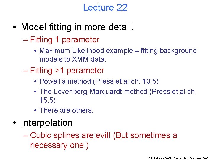
Lecture 22 • Model fitting in more detail. – Fitting 1 parameter • Maximum Likelihood example – fitting background models to XMM data. – Fitting >1 parameter • Powell’s method (Press et al ch. 10. 5) • The Levenberg-Marquardt method (Press et al ch. 15. 5) • There are others. • Interpolation – Cubic splines are evil! (But sometimes a necessary one. ) NASSP Masters 5003 F - Computational Astronomy - 2009

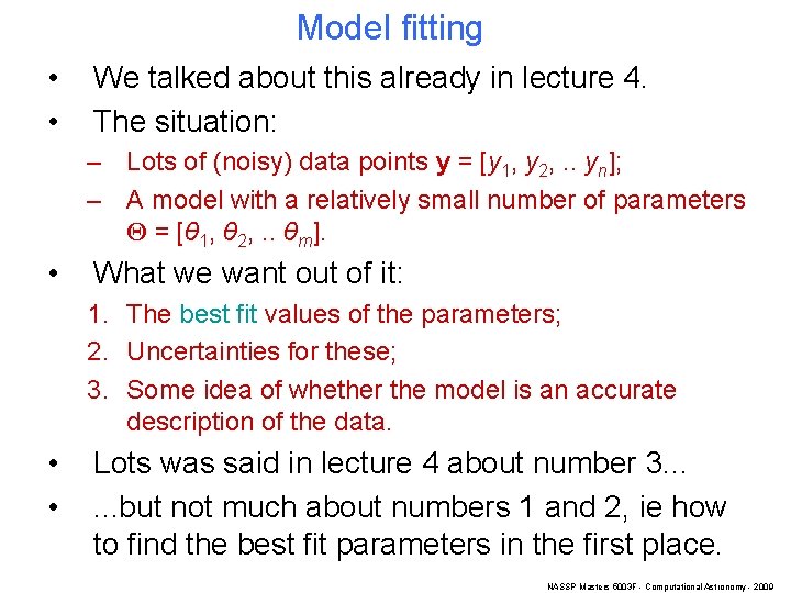
Model fitting • • We talked about this already in lecture 4. The situation: – Lots of (noisy) data points y = [y 1, y 2, . . yn]; – A model with a relatively small number of parameters Θ = [θ 1, θ 2, . . θm]. • What we want out of it: 1. The best fit values of the parameters; 2. Uncertainties for these; 3. Some idea of whether the model is an accurate description of the data. • • Lots was said in lecture 4 about number 3. . . but not much about numbers 1 and 2, ie how to find the best fit parameters in the first place. NASSP Masters 5003 F - Computational Astronomy - 2009

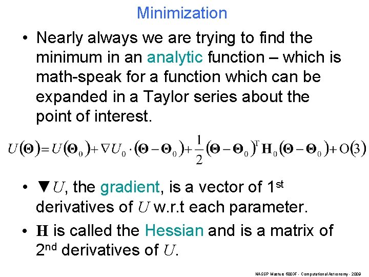
Minimization • Nearly always we are trying to find the minimum in an analytic function – which is math-speak for a function which can be expanded in a Taylor series about the point of interest. • ▼U, the gradient, is a vector of 1 st derivatives of U w. r. t each parameter. • H is called the Hessian and is a matrix of 2 nd derivatives of U. NASSP Masters 5003 F - Computational Astronomy - 2009

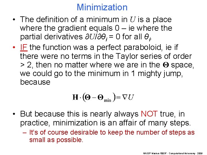
Minimization • The definition of a minimum in U is a place where the gradient equals 0 – ie where the partial derivatives ∂U/∂θi = 0 for all θi. • IF the function was a perfect paraboloid, ie if there were no terms in the Taylor series of order > 2, then no matter where we are in the Θ space, we could go to the minimum in 1 mighty jump, because • But because this is nearly always NOT true, in practice, minimization is an affair of many steps. – It’s of course desirable to keep the number of steps as small as possible. NASSP Masters 5003 F - Computational Astronomy - 2009

Minimization issues: 1. Robust setting of starting bounds: how to make sure the minimum is within the box. • • • Once you know that, you can, in the words of Press et al, “hunt it down like a scared rabbit. ” For only 1 parameter, there algorithms to find a bracket which must contain the minimum (Press et al ch. 10. 1). This is more difficult to arrange in more than 1 dimension because one has then to deal with a bounding surface, possibly of complicated shape, rather than 2 scalar values. 2. Speed – if you have to find a series of minima in multi-dimensional functions, a good choice of algorithm (and its settings) can give a valuable speed dividend. • Eg the XMM-Newton source fitting task – fits 7 or more parameters per source – it’s one of the slowest tasks in the pipeline. Could have been a lot worse though with a poor choice of algorithm (it uses Levenberg-Marquardt). NASSP Masters 5003 F - Computational Astronomy - 2009

Minimization issues: 3. Stability. • There is often a trade-off between speed and stability. 4. When to stop – ie convergence tests. • Basically the time to stop is when the step size per iteration is smaller than the dimensions of the uncertainty ellipsoid. 5. Is it a local minimum or a global one? • • Many algorithms will be perfectly happy stopping in a tiny local dip in the function. Extra intelligence is needed to hunt around and make sure your minimum is the best in the neighbourhood. Annealing algorithms. NASSP Masters 5003 F - Computational Astronomy - 2009

Minimization with 1 parameter • Algorithm depends on whether ∂U/∂θ and higher derivatives are calculable or not. I use: – If yes, Newton-Raphson method. – If no, Brent’s method (Press et al ch 10. 2). This consists of: • Parabolic fit if this is well-behaved; • Golden-section search when not. NASSP Masters 5003 F - Computational Astronomy - 2009

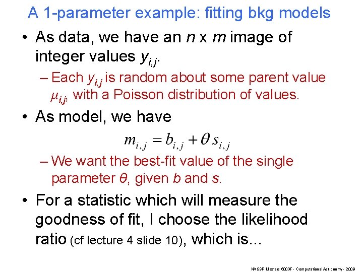
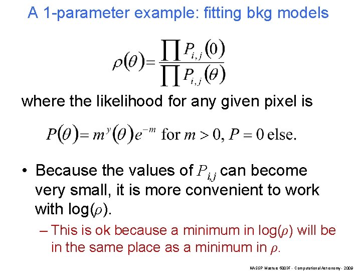
A 1 -parameter example: fitting bkg models • As data, we have an n x m image of integer values yi, j. – Each yi, j is random about some parent value μi, j, with a Poisson distribution of values. • As model, we have – We want the best-fit value of the single parameter θ, given b and s. • For a statistic which will measure the goodness of fit, I choose the likelihood ratio (cf lecture 4 slide 10), which is. . . NASSP Masters 5003 F - Computational Astronomy - 2009

A 1 -parameter example: fitting bkg models where the likelihood for any given pixel is • Because the values of Pi, j can become very small, it is more convenient to work with log(ρ). – This is ok because a minimum in log(ρ) will be in the same place as a minimum in ρ. NASSP Masters 5003 F - Computational Astronomy - 2009

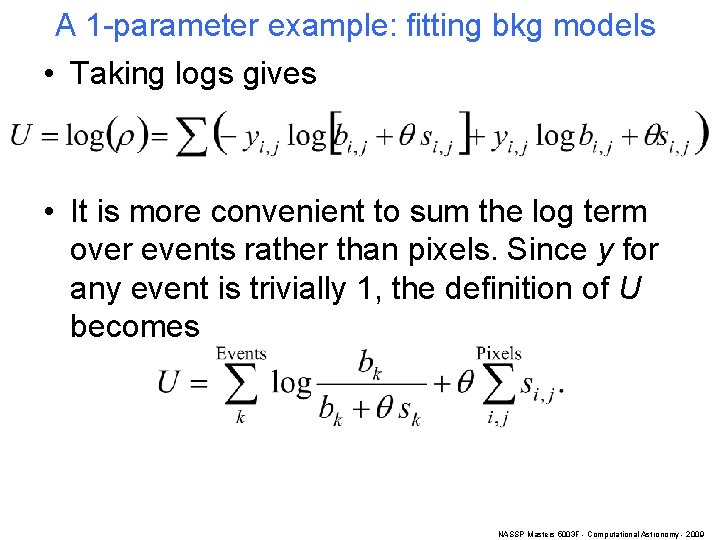
A 1 -parameter example: fitting bkg models • Taking logs gives • It is more convenient to sum the log term over events rather than pixels. Since y for any event is trivially 1, the definition of U becomes NASSP Masters 5003 F - Computational Astronomy - 2009

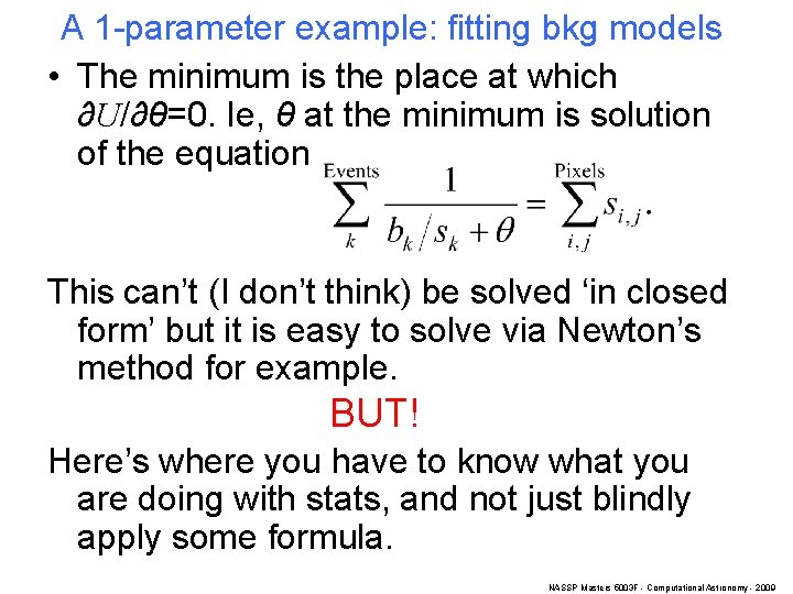
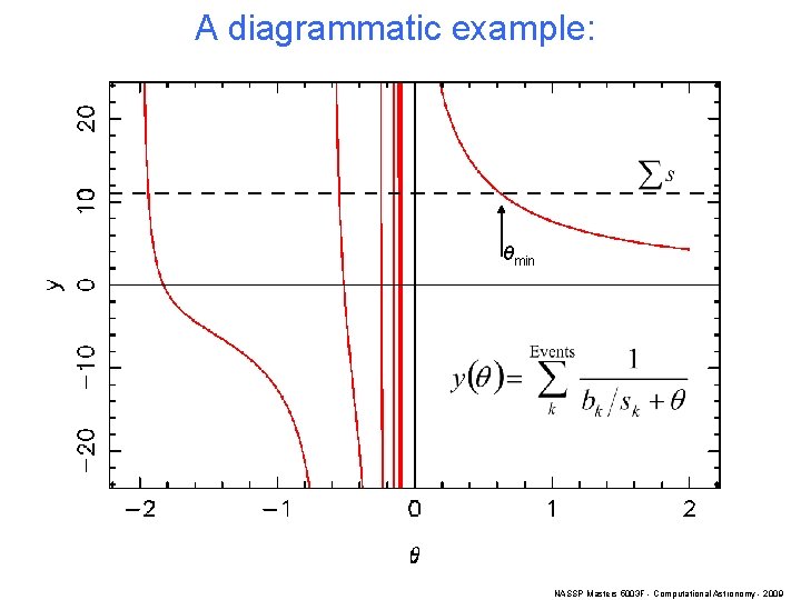
A 1 -parameter example: fitting bkg models • The minimum is the place at which ∂U/∂θ=0. Ie, θ at the minimum is solution of the equation This can’t (I don’t think) be solved ‘in closed form’ but it is easy to solve via Newton’s method for example. BUT! Here’s where you have to know what you are doing with stats, and not just blindly apply some formula. NASSP Masters 5003 F - Computational Astronomy - 2009

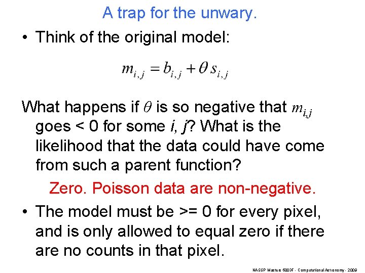
A trap for the unwary. • Think of the original model: What happens if θ is so negative that mi, j goes < 0 for some i, j? What is the likelihood that the data could have come from such a parent function? Zero. Poisson data are non-negative. • The model must be >= 0 for every pixel, and is only allowed to equal zero if there are no counts in that pixel. NASSP Masters 5003 F - Computational Astronomy - 2009

A diagrammatic example: θmin NASSP Masters 5003 F - Computational Astronomy - 2009

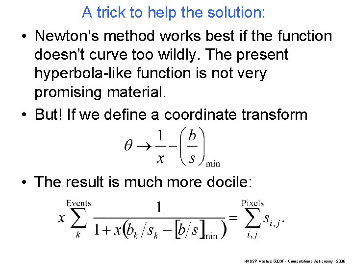
A trick to help the solution: • Newton’s method works best if the function doesn’t curve too wildly. The present hyperbola-like function is not very promising material. • But! If we define a coordinate transform • The result is much more docile: NASSP Masters 5003 F - Computational Astronomy - 2009

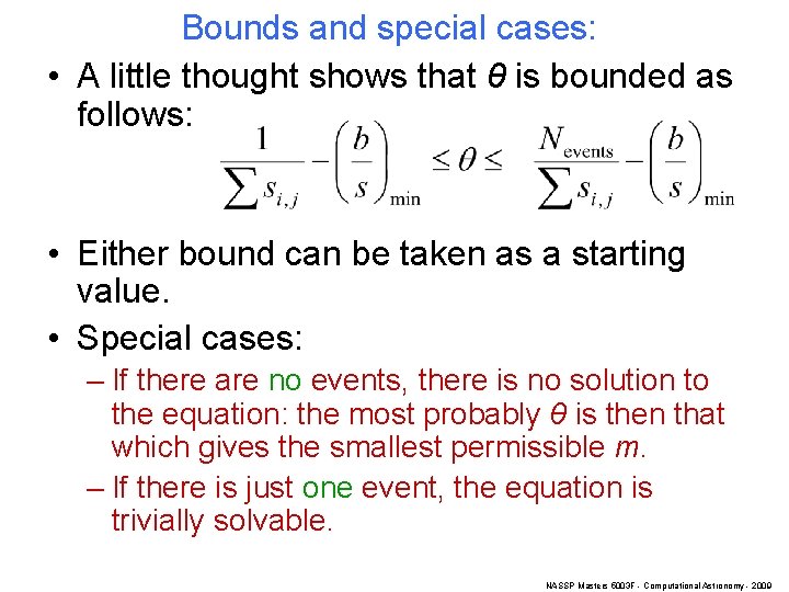
Bounds and special cases: • A little thought shows that θ is bounded as follows: • Either bound can be taken as a starting value. • Special cases: – If there are no events, there is no solution to the equation: the most probably θ is then that which gives the smallest permissible m. – If there is just one event, the equation is trivially solvable. NASSP Masters 5003 F - Computational Astronomy - 2009

Minimization with >1 parameter • The basic idea is to 1. Measure the gradient, 2. then head down-hill. You’re bound to hit at least a local minimum eventually. • But how far should you go at each step, before stopping to sample U and ▼U again? – – • Suppose you find you gone wayyy too far - have climbed through a gully and higher up the opposite wall than the height you started? Or suppose you have only crept a few inches down a slope which seems to extend for miles? Solution: treat each direction like a 1 -D minimization. NASSP Masters 5003 F - Computational Astronomy - 2009

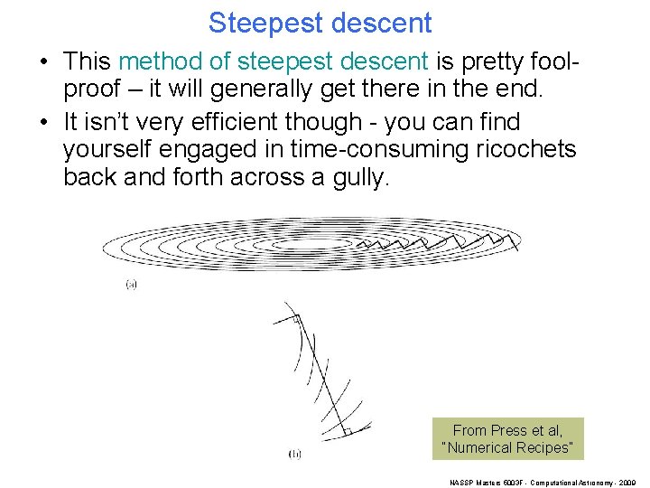
Steepest descent • This method of steepest descent is pretty foolproof – it will generally get there in the end. • It isn’t very efficient though - you can find yourself engaged in time-consuming ricochets back and forth across a gully. From Press et al, “Numerical Recipes” NASSP Masters 5003 F - Computational Astronomy - 2009

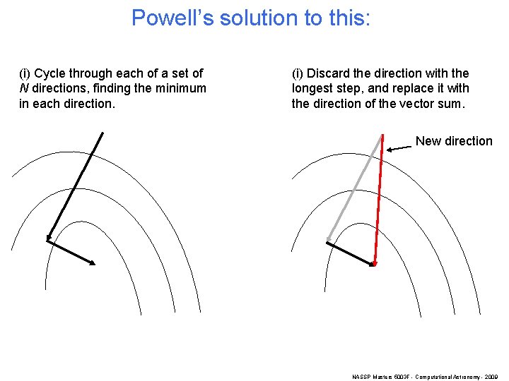
Powell’s solution to this: (i) Cycle through each of a set of N directions, finding the minimum in each direction. (i) Discard the direction with the longest step, and replace it with the direction of the vector sum. New direction NASSP Masters 5003 F - Computational Astronomy - 2009

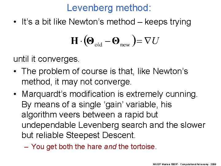
Levenberg method: • It’s a bit like Newton’s method – keeps trying until it converges. • The problem of course is that, like Newton’s method, it may not converge. • Marquardt’s modification is extremely cunning. By means of a single ‘gain’ variable, his algorithm veers between a rapid but undependable Levenberg search and the slower but reliable Steepest Descent. – You get both the hare and the tortoise. NASSP Masters 5003 F - Computational Astronomy - 2009

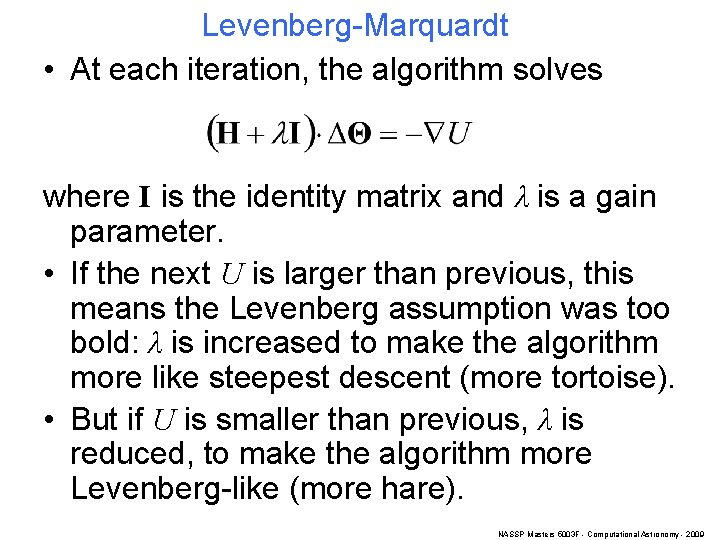
Levenberg-Marquardt • At each iteration, the algorithm solves where I is the identity matrix and λ is a gain parameter. • If the next U is larger than previous, this means the Levenberg assumption was too bold: λ is increased to make the algorithm more like steepest descent (more tortoise). • But if U is smaller than previous, λ is reduced, to make the algorithm more Levenberg-like (more hare). NASSP Masters 5003 F - Computational Astronomy - 2009

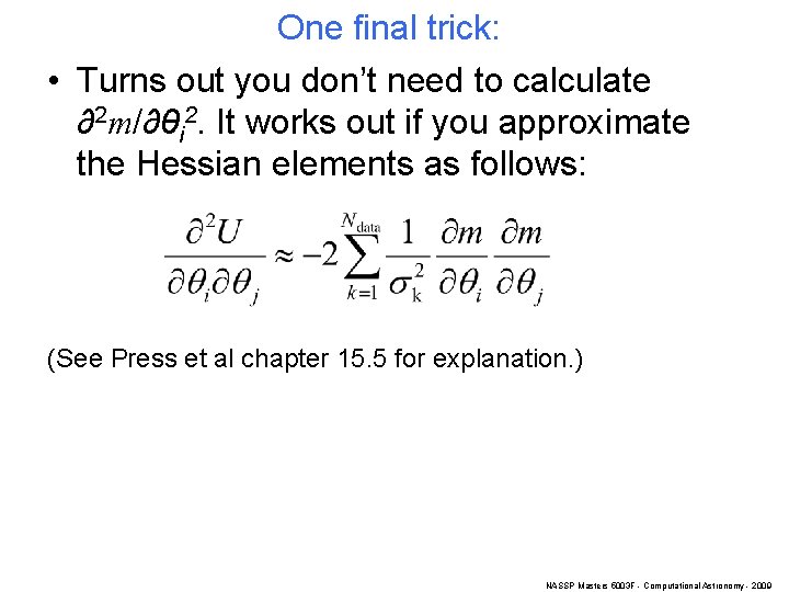
One final trick: • Turns out you don’t need to calculate ∂2 m/∂θi 2. It works out if you approximate the Hessian elements as follows: (See Press et al chapter 15. 5 for explanation. ) NASSP Masters 5003 F - Computational Astronomy - 2009

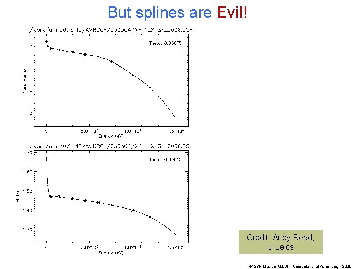
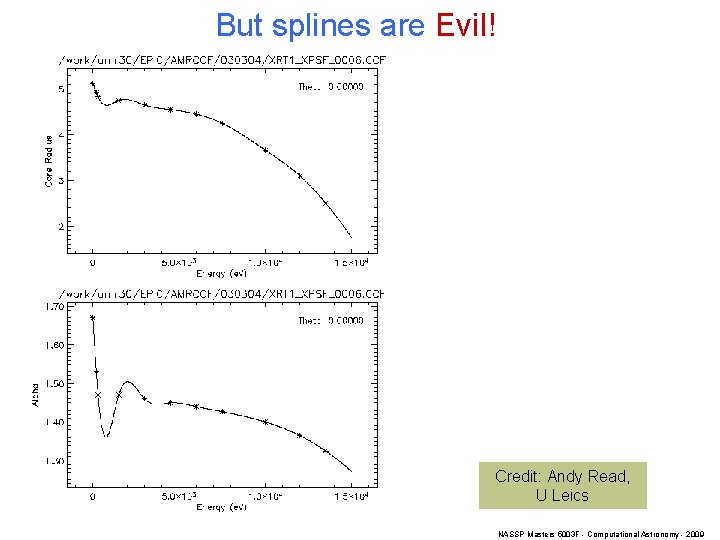
Interpolation • The difference between interpolation and fitting is the comparison between the number Npar of parameters number Ndata of data points. – If Ndata > Npar, you fit. – If Ndata = Npar, you interpolate. – If Ndata < Npar, you either kill off some parameters. . . or resort to Bayesian black magic. • Because interpolation is only loosely constrained by the data (think of a strait jacket with most of the buttons undone), it can be unstable. See eg in a few slides. NASSP Masters 5003 F - Computational Astronomy - 2009

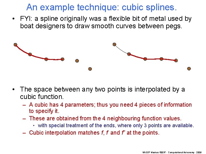
An example technique: cubic splines. • FYI: a spline originally was a flexible bit of metal used by boat designers to draw smooth curves between pegs. • The space between any two points is interpolated by a cubic function. – A cubic has 4 parameters; thus you need 4 pieces of information to specify it. – These are obtained from the 4 neighbouring function values. • with special treatment of the ends, where only 3 points are available. – Cubic interpolation matches f, f’ and f” at the points. NASSP Masters 5003 F - Computational Astronomy - 2009

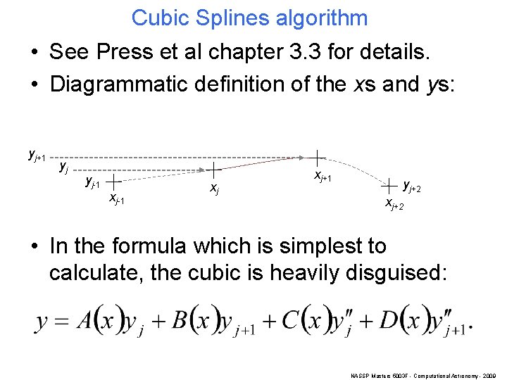
Cubic Splines algorithm • See Press et al chapter 3. 3 for details. • Diagrammatic definition of the xs and ys: yj+1 yj yj-1 xj xj+1 yj+2 xj+2 • In the formula which is simplest to calculate, the cubic is heavily disguised: NASSP Masters 5003 F - Computational Astronomy - 2009

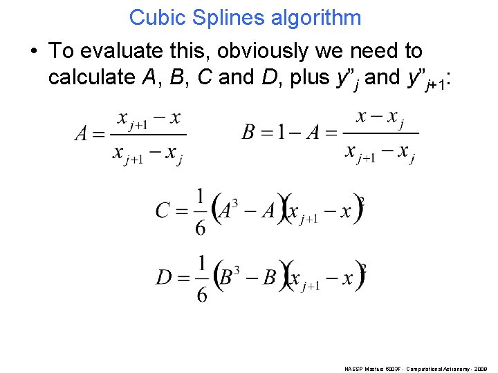
Cubic Splines algorithm • To evaluate this, obviously we need to calculate A, B, C and D, plus y”j and y”j+1: NASSP Masters 5003 F - Computational Astronomy - 2009

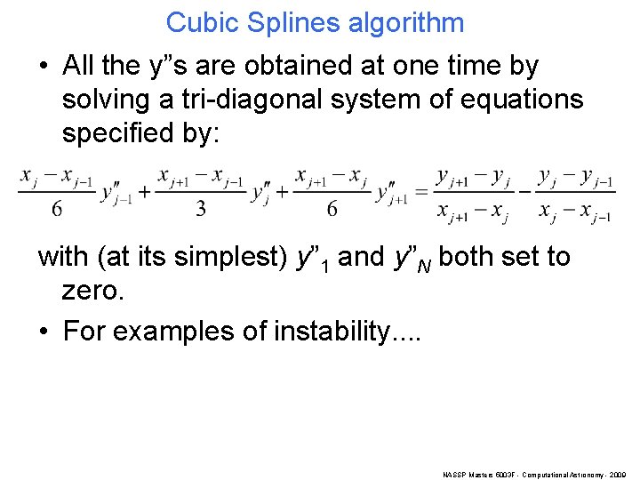
Cubic Splines algorithm • All the y”s are obtained at one time by solving a tri-diagonal system of equations specified by: with (at its simplest) y” 1 and y”N both set to zero. • For examples of instability. . NASSP Masters 5003 F - Computational Astronomy - 2009

But splines are Evil! Credit: Andy Read, U Leics NASSP Masters 5003 F - Computational Astronomy - 2009

But splines are Evil! Credit: Andy Read, U Leics NASSP Masters 5003 F - Computational Astronomy - 2009