12 Simple Linear Regression and Correlation Copyright Cengage

12 Simple Linear Regression and Correlation Copyright © Cengage Learning. All rights reserved.

12. 3 Inferences About the Slope Parameter 1 Copyright © Cengage Learning. All rights reserved.

Inferences About the Slope Parameter 1 In virtually all of our inferential work thus far, the notion of sampling variability has been pervasive. In particular, properties of sampling distributions of various statistics have been the basis for developing confidence interval formulas and hypothesis-testing methods. The key idea here is that the value of any quantity calculated from sample data—the value of any statistic—will vary from one sample to another. 3

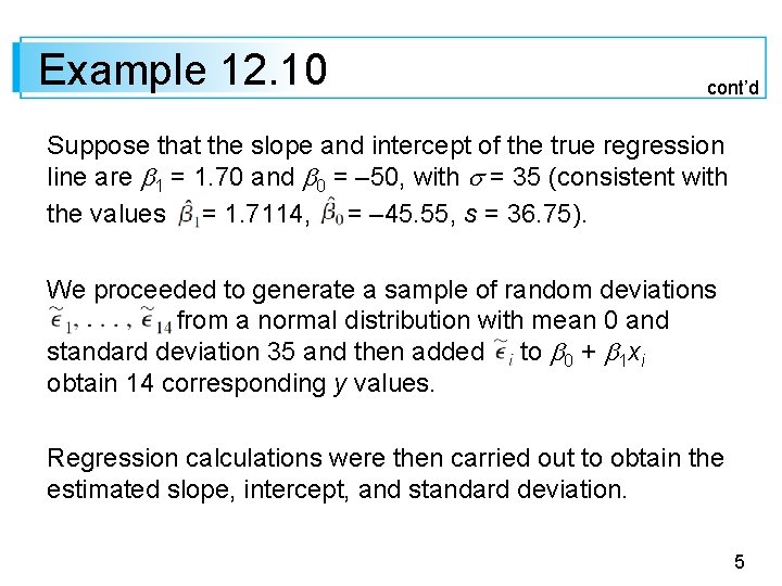
Example 12. 10 Reconsider the data on x = burner-area liberation rate and y = NOx emission rate from Exercise 12. 19 in the pervious section. There are 14 observations, made at the x values 100, 125, 150, 200, 250, 300, 350, 400, and 400, respectively. 4

Example 12. 10 cont’d Suppose that the slope and intercept of the true regression line are 1 = 1. 70 and 0 = – 50, with = 35 (consistent with the values = 1. 7114, = – 45. 55, s = 36. 75). We proceeded to generate a sample of random deviations from a normal distribution with mean 0 and standard deviation 35 and then added to 0 + 1 xi obtain 14 corresponding y values. Regression calculations were then carried out to obtain the estimated slope, intercept, and standard deviation. 5

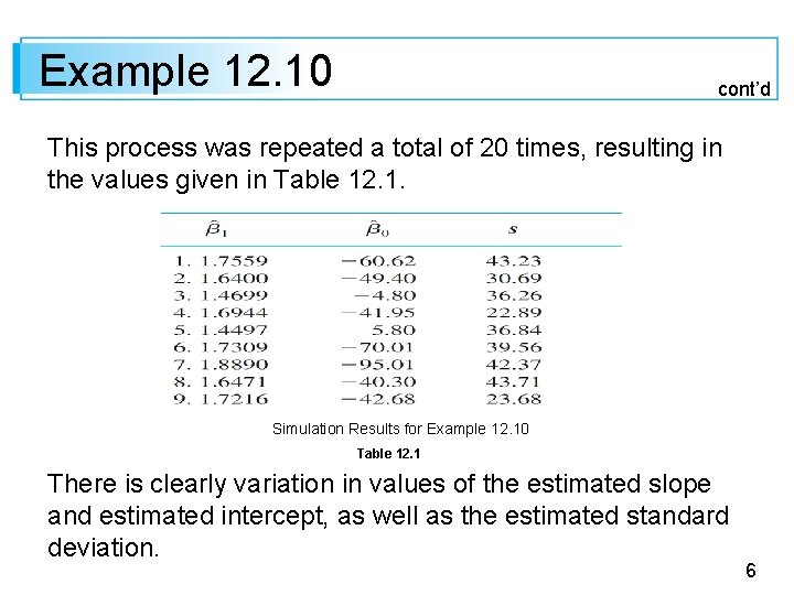
Example 12. 10 cont’d This process was repeated a total of 20 times, resulting in the values given in Table 12. 1. Simulation Results for Example 12. 10 Table 12. 1 There is clearly variation in values of the estimated slope and estimated intercept, as well as the estimated standard deviation. 6

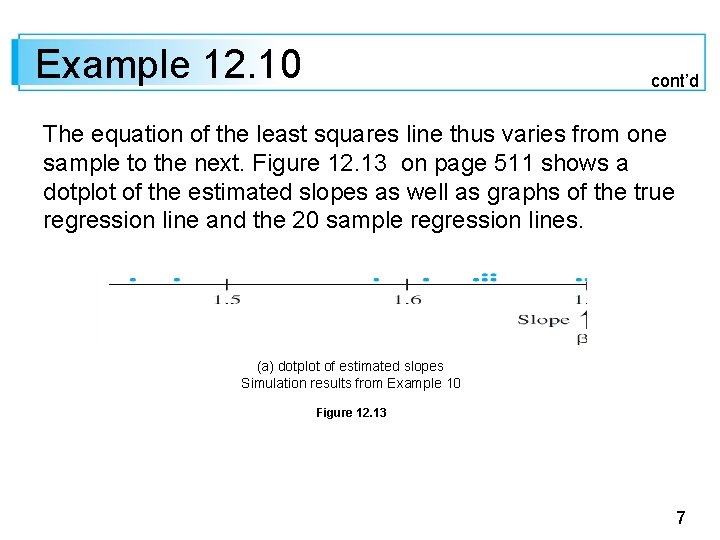
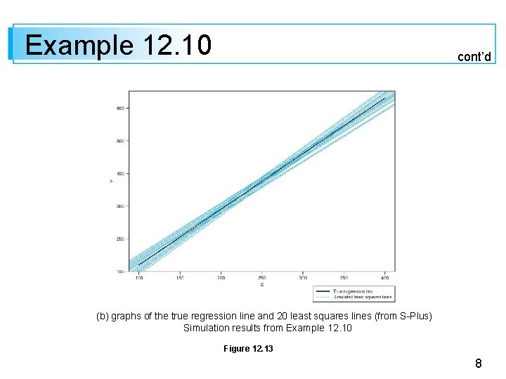
Example 12. 10 cont’d The equation of the least squares line thus varies from one sample to the next. Figure 12. 13 on page 511 shows a dotplot of the estimated slopes as well as graphs of the true regression line and the 20 sample regression lines. (a) dotplot of estimated slopes Simulation results from Example 10 Figure 12. 13 7

Example 12. 10 cont’d (b) graphs of the true regression line and 20 least squares lines (from S-Plus) Simulation results from Example 12. 10 Figure 12. 13 8

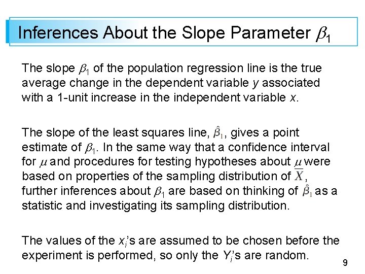
Inferences About the Slope Parameter 1 The slope 1 of the population regression line is the true average change in the dependent variable y associated with a 1 -unit increase in the independent variable x. The slope of the least squares line, , gives a point estimate of 1. In the same way that a confidence interval for and procedures for testing hypotheses about were based on properties of the sampling distribution of , further inferences about 1 are based on thinking of as a statistic and investigating its sampling distribution. The values of the xi’s are assumed to be chosen before the experiment is performed, so only the Yi’s are random. 9

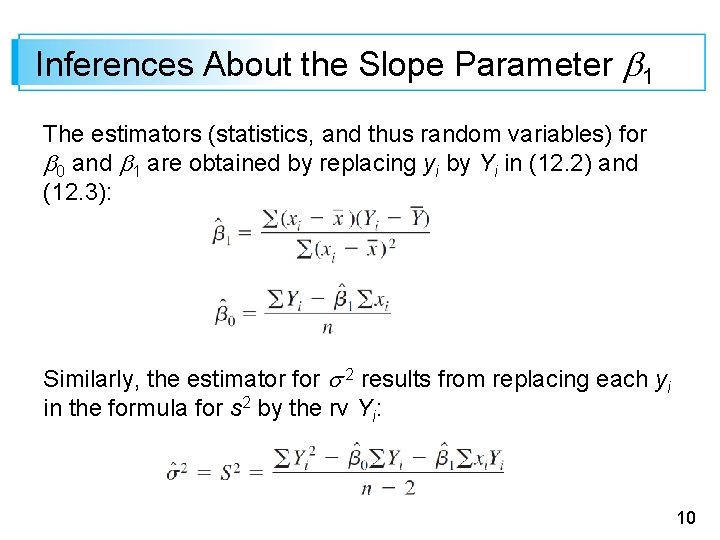
Inferences About the Slope Parameter 1 The estimators (statistics, and thus random variables) for 0 and 1 are obtained by replacing yi by Yi in (12. 2) and (12. 3): Similarly, the estimator for 2 results from replacing each yi in the formula for s 2 by the rv Yi: 10

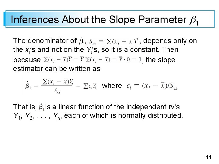
Inferences About the Slope Parameter 1 The denominator of , , depends only on the xi’s and not on the Yi’s, so it is a constant. Then because , the slope estimator can be written as where That is, is a linear function of the independent rv’s Y 1, Y 2, . . . , Yn, each of which is normally distributed. 11

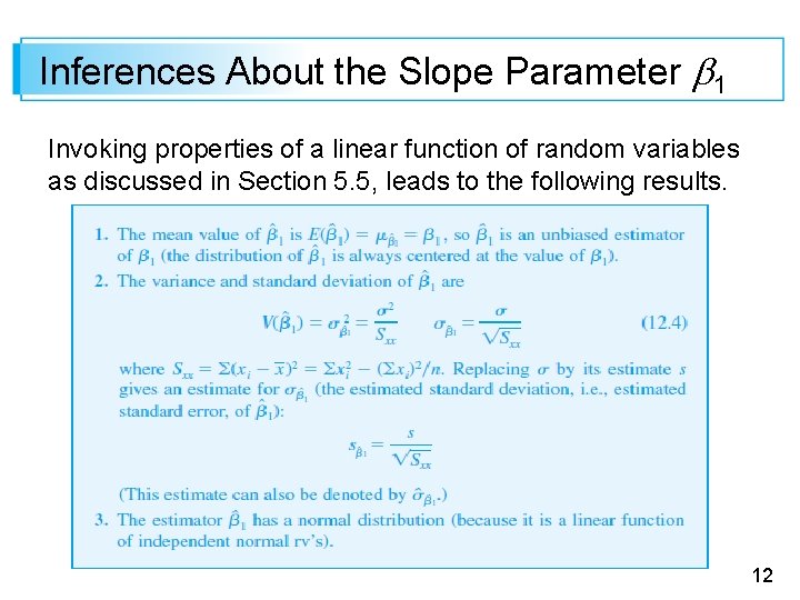
Inferences About the Slope Parameter 1 Invoking properties of a linear function of random variables as discussed in Section 5. 5, leads to the following results. 12

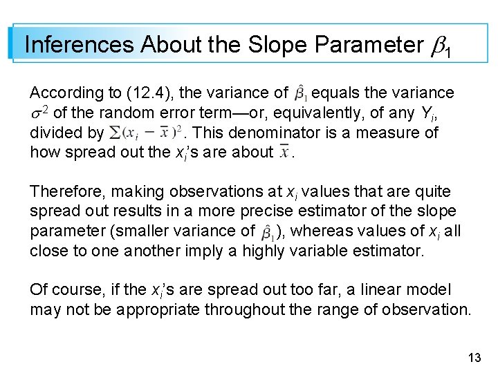
Inferences About the Slope Parameter 1 According to (12. 4), the variance of equals the variance 2 of the random error term—or, equivalently, of any Yi, divided by. This denominator is a measure of how spread out the xi’s are about. Therefore, making observations at xi values that are quite spread out results in a more precise estimator of the slope parameter (smaller variance of ), whereas values of xi all close to one another imply a highly variable estimator. Of course, if the xi’s are spread out too far, a linear model may not be appropriate throughout the range of observation. 13

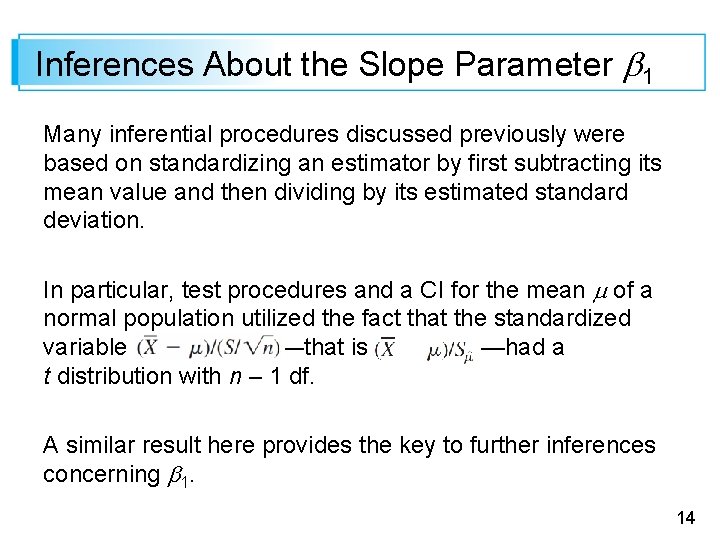
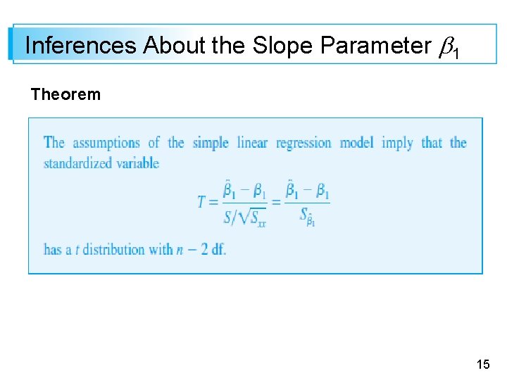
Inferences About the Slope Parameter 1 Many inferential procedures discussed previously were based on standardizing an estimator by first subtracting its mean value and then dividing by its estimated standard deviation. In particular, test procedures and a CI for the mean of a normal population utilized the fact that the standardized variable —that is —had a t distribution with n – 1 df. A similar result here provides the key to further inferences concerning 1. 14

Inferences About the Slope Parameter 1 Theorem 15

A Confidence Interval for 1 16

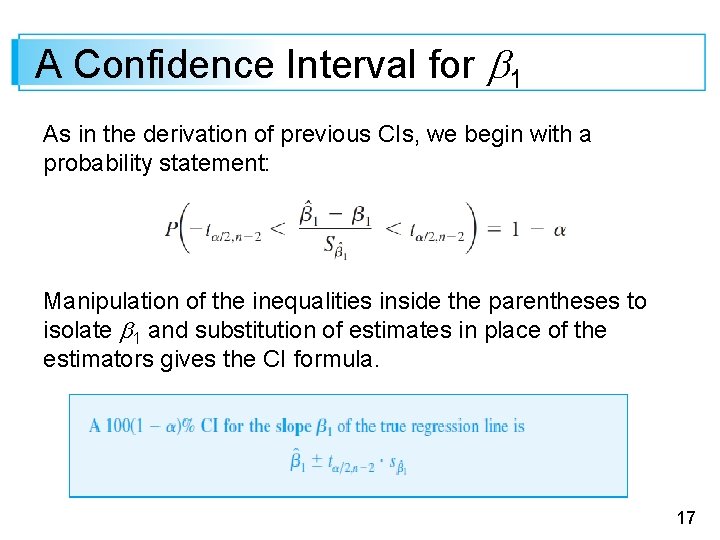
A Confidence Interval for 1 As in the derivation of previous CIs, we begin with a probability statement: Manipulation of the inequalities inside the parentheses to isolate 1 and substitution of estimates in place of the estimators gives the CI formula. 17

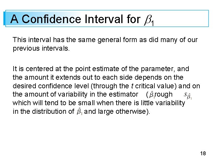
A Confidence Interval for 1 This interval has the same general form as did many of our previous intervals. It is centered at the point estimate of the parameter, and the amount it extends out to each side depends on the desired confidence level (through the t critical value) and on the amount of variability in the estimator (through , which will tend to be small when there is little variability in the distribution of and large otherwise). 18

Example 12. 11 When damage to a timber structure occurs, it may be more economical to repair the damaged area rather than replace the entire structure. The article “Simplified Model for Strength Assessment of Timber Beams Joined by Bonded Plates” (J. of Materials in Civil Engr. , 2013: 980– 990) investigated a particular strategy for repair. The accompanying data was used by the authors of the article as a basis for fitting the simple linear regression model. 19

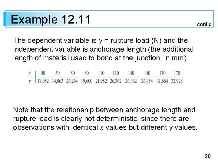
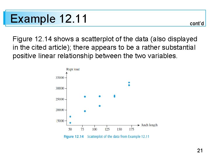
Example 12. 11 cont’d The dependent variable is y = rupture load (N) and the independent variable is anchorage length (the additional length of material used to bond at the junction, in mm). Note that the relationship between anchorage length and rupture load is clearly not deterministic, since there are observations with identical x values but different y values. 20

Example 12. 11 cont’d Figure 12. 14 shows a scatterplot of the data (also displayed in the cited article); there appears to be a rather substantial positive linear relationship between the two variables. 21

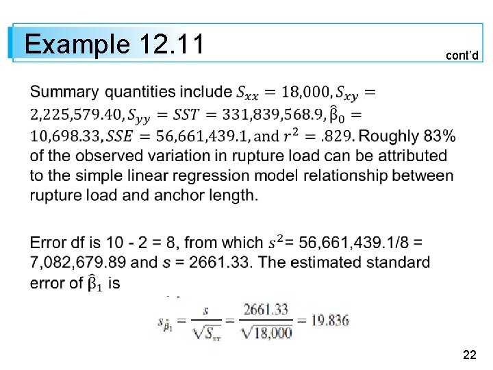
Example 12. 11 cont’d 22

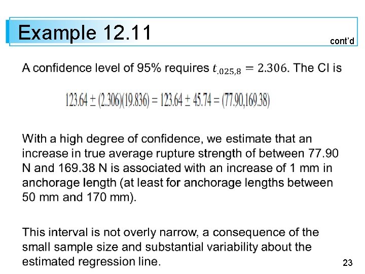
Example 12. 11 cont’d 23

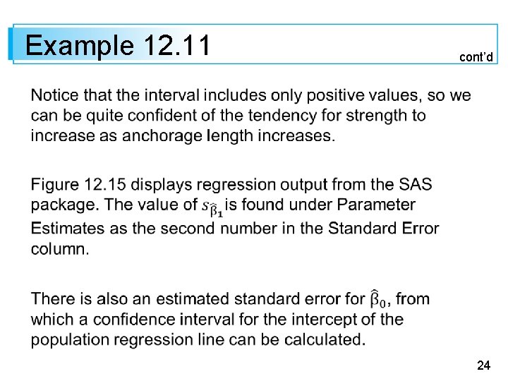
Example 12. 11 cont’d 24

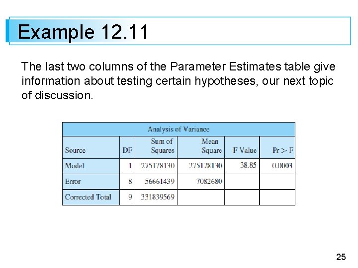
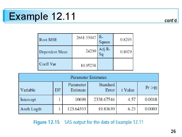
Example 12. 11 The last two columns of the Parameter Estimates table give information about testing certain hypotheses, our next topic of discussion. 25

Example 12. 11 cont’d 26

Hypothesis-Testing Procedures 27

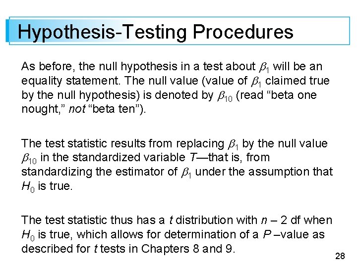
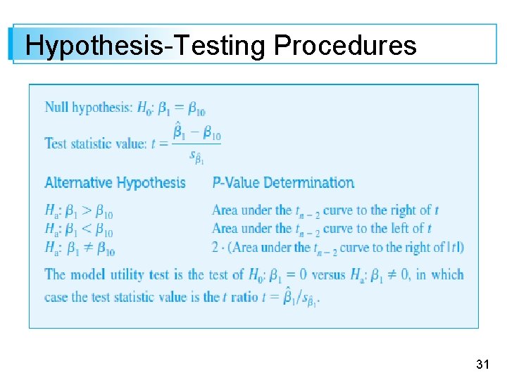
Hypothesis-Testing Procedures As before, the null hypothesis in a test about 1 will be an equality statement. The null value (value of 1 claimed true by the null hypothesis) is denoted by 10 (read “beta one nought, ” not “beta ten”). The test statistic results from replacing 1 by the null value 10 in the standardized variable T—that is, from standardizing the estimator of 1 under the assumption that H 0 is true. The test statistic thus has a t distribution with n – 2 df when H 0 is true, which allows for determination of a P –value as described for t tests in Chapters 8 and 9. 28

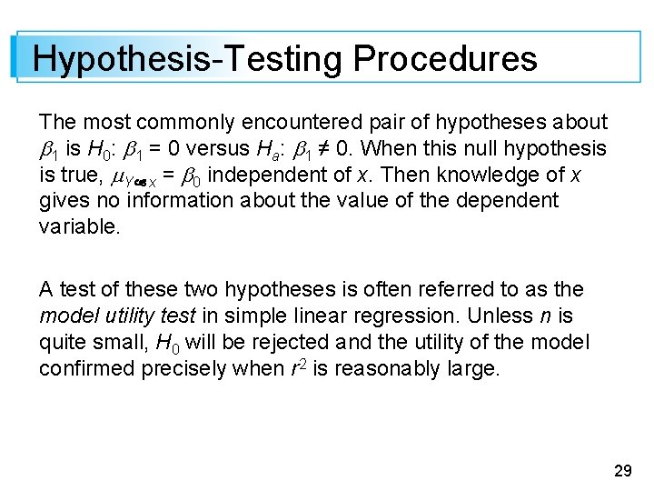
Hypothesis-Testing Procedures The most commonly encountered pair of hypotheses about 1 is H 0: 1 = 0 versus Ha: 1 ≠ 0. When this null hypothesis is true, Y x = 0 independent of x. Then knowledge of x gives no information about the value of the dependent variable. A test of these two hypotheses is often referred to as the model utility test in simple linear regression. Unless n is quite small, H 0 will be rejected and the utility of the model confirmed precisely when r 2 is reasonably large. 29

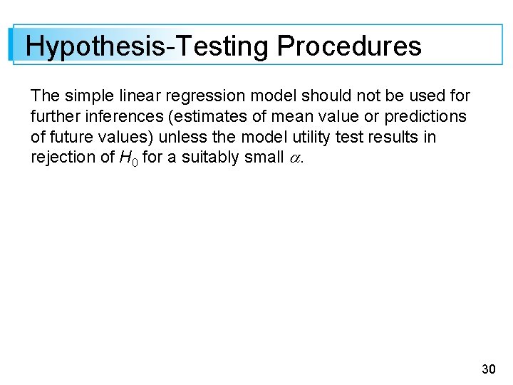
Hypothesis-Testing Procedures The simple linear regression model should not be used for further inferences (estimates of mean value or predictions of future values) unless the model utility test results in rejection of H 0 for a suitably small . 30

Hypothesis-Testing Procedures 31

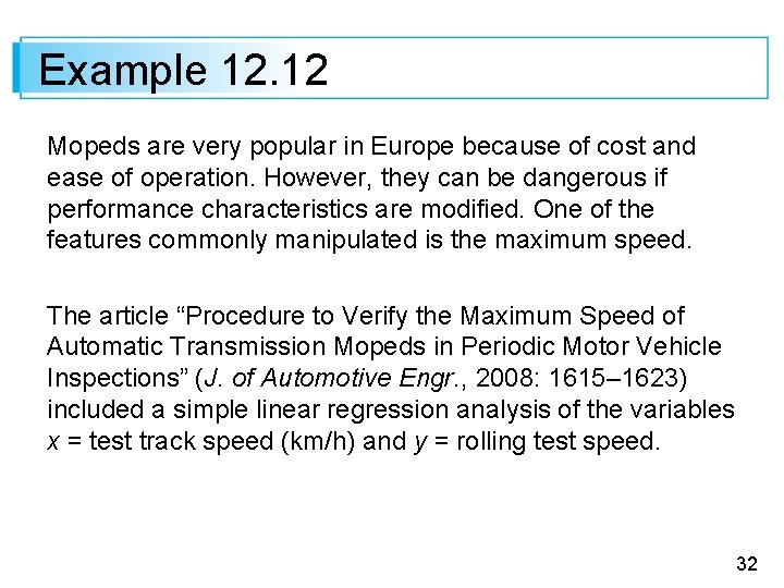
Example 12. 12 Mopeds are very popular in Europe because of cost and ease of operation. However, they can be dangerous if performance characteristics are modified. One of the features commonly manipulated is the maximum speed. The article “Procedure to Verify the Maximum Speed of Automatic Transmission Mopeds in Periodic Motor Vehicle Inspections” (J. of Automotive Engr. , 2008: 1615– 1623) included a simple linear regression analysis of the variables x = test track speed (km/h) and y = rolling test speed. 32

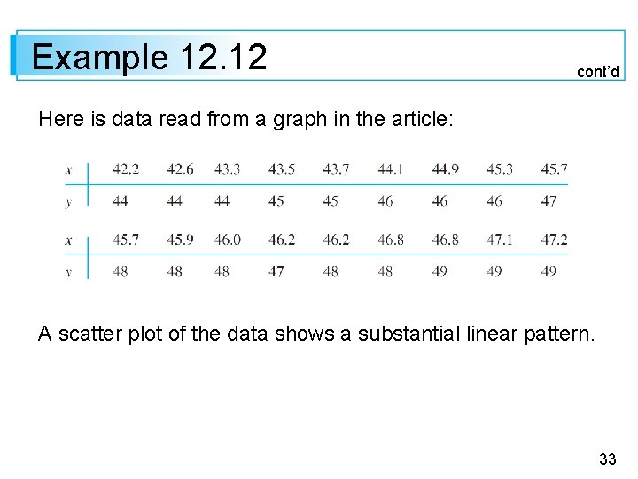
Example 12. 12 cont’d Here is data read from a graph in the article: A scatter plot of the data shows a substantial linear pattern. 33

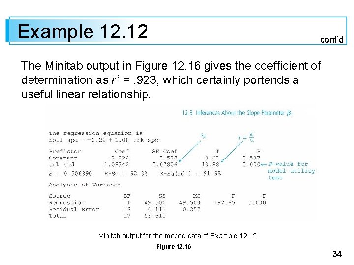
Example 12. 12 cont’d The Minitab output in Figure 12. 16 gives the coefficient of determination as r 2 =. 923, which certainly portends a useful linear relationship. Minitab output for the moped data of Example 12. 12 Figure 12. 16 34

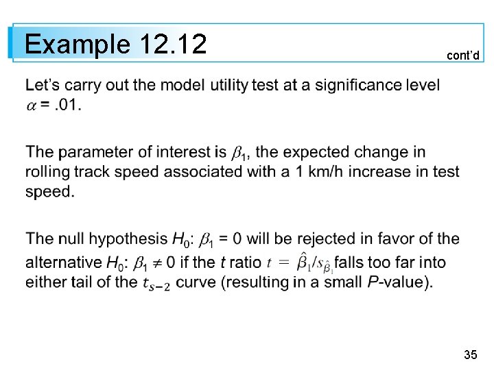
Example 12. 12 cont’d 35

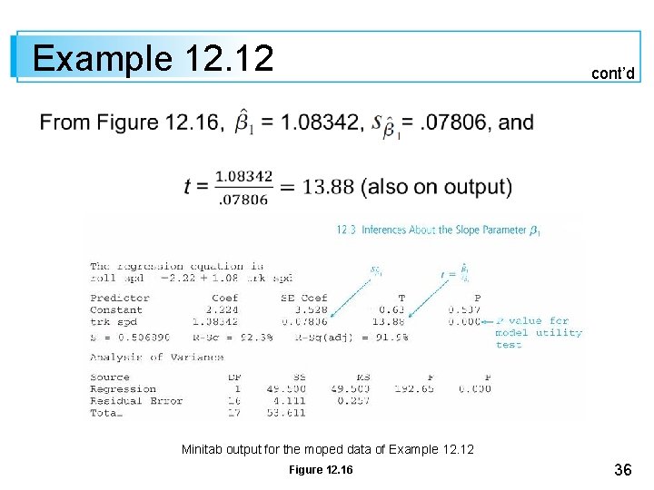
Example 12. 12 cont’d Minitab output for the moped data of Example 12. 12 Figure 12. 16 36

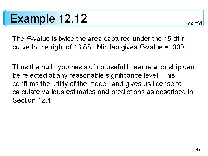
Example 12. 12 cont’d The P-value is twice the area captured under the 16 df t curve to the right of 13. 88. Minitab gives P-value =. 000. Thus the null hypothesis of no useful linear relationship can be rejected at any reasonable significance level. This confirms the utility of the model, and gives us license to calculate various estimates and predictions as described in Section 12. 4. 37

Regression and ANOVA 38

Regression and ANOVA The decomposition of the total sum of squares into a part SSE, which measures unexplained variation, and a part SSR, which measures variation explained by the linear relationship, is strongly reminiscent of one-way ANOVA. 39

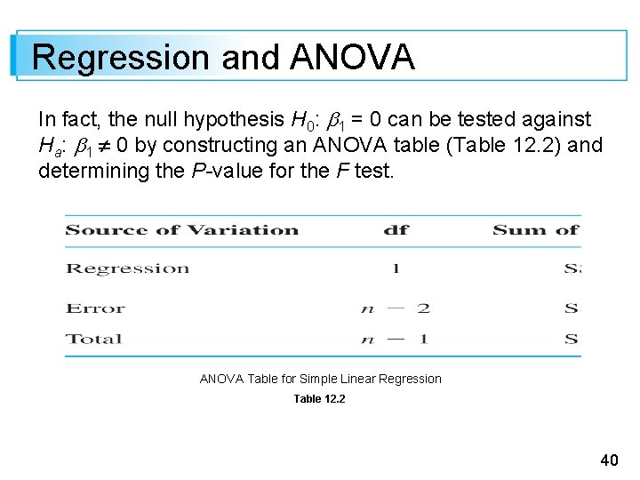
Regression and ANOVA In fact, the null hypothesis H 0: 1 = 0 can be tested against Ha: 1 0 by constructing an ANOVA table (Table 12. 2) and determining the P-value for the F test. ANOVA Table for Simple Linear Regression Table 12. 2 40

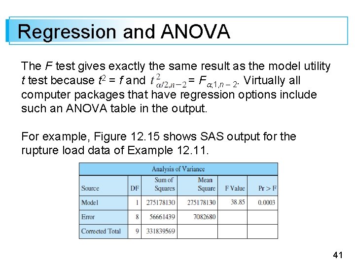
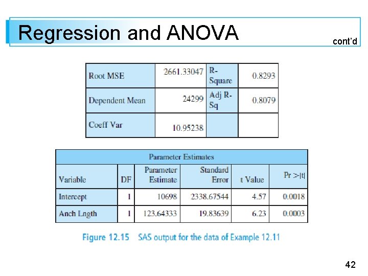
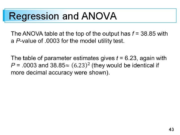
Regression and ANOVA The F test gives exactly the same result as the model utility t test because t 2 = f and = F , 1, n – 2. Virtually all computer packages that have regression options include such an ANOVA table in the output. For example, Figure 12. 15 shows SAS output for the rupture load data of Example 12. 11. 41

Regression and ANOVA cont’d 42

Regression and ANOVA 43