12 Simple Linear Regression and Correlation Copyright Cengage

12 Simple Linear Regression and Correlation Copyright © Cengage Learning. All rights reserved.

12. 2 Estimating Model Parameters Copyright © Cengage Learning. All rights reserved.

Estimating Model Parameters We will assume in this and the next several sections that the variables x and y are related according to the simple linear regression model. The values of 0, 1, and 2 will almost never be known to an investigator. Instead, sample data consisting of n observed pairs (x 1, y 1), …, (xn, yn) will be available, from which the model parameters and the true regression line itself can be estimated. These observations are assumed to have been obtained independently of one another. 3

Estimating Model Parameters That is, yi is the observed value of Yi, where Yi = 0 + 1 xi + I and the n deviations 1, 2, …, n are independent rv’s. Independence of Y 1, Y 2, …, Yn follows from independence of the i’s. According to the model, the observed points will be distributed about the true regression line in a random manner. 4

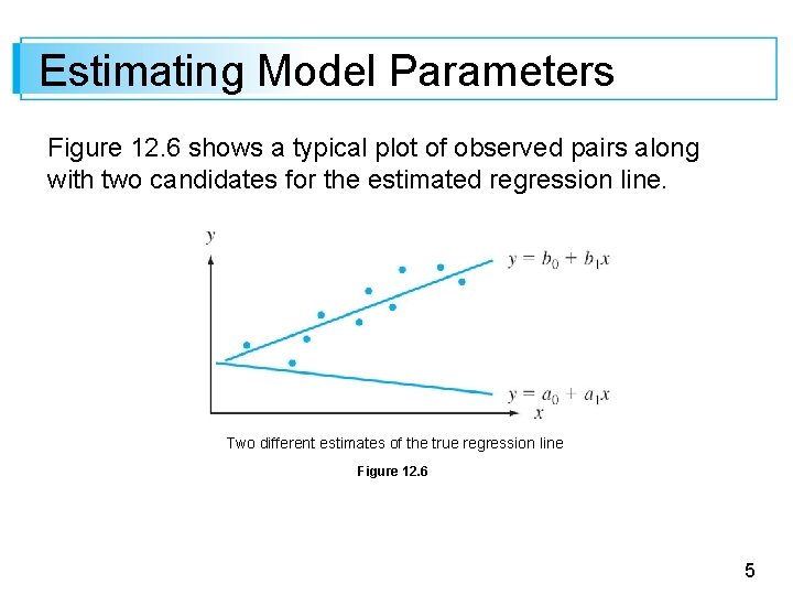
Estimating Model Parameters Figure 12. 6 shows a typical plot of observed pairs along with two candidates for the estimated regression line. Two different estimates of the true regression line Figure 12. 6 5

Estimating Model Parameters Intuitively, the line y = a 0 + a 1 x is not a reasonable estimate of the true line y = 0 + 1 x because, if y = a 0 + a 1 x were the true line, the observed points would almost surely have been closer to this line. The line y = b 0 + b 1 x is a more plausible estimate because the observed points are scattered rather closely about this line. Figure 12. 6 and the foregoing discussion suggest that our estimate of y = 0 + 1 x should be a line that provides in some sense a best fit to the observed data points. 6

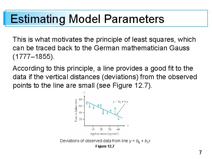
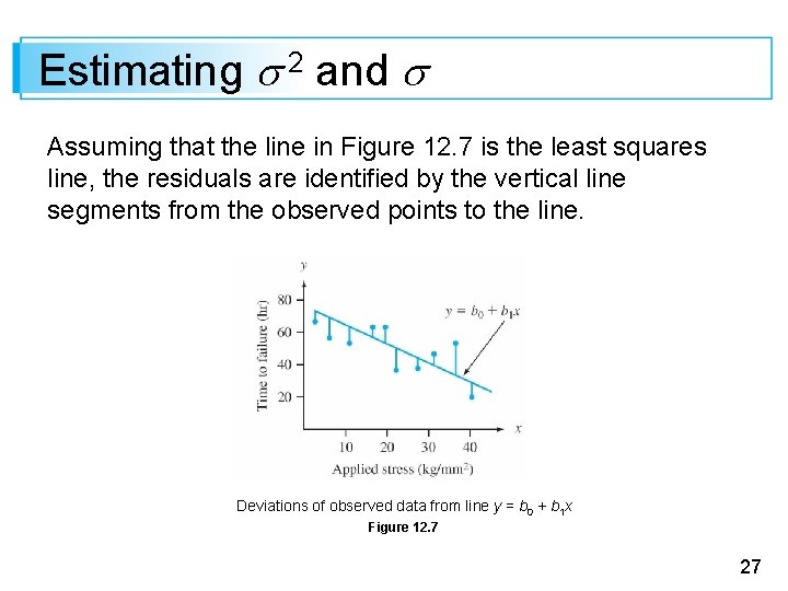
Estimating Model Parameters This is what motivates the principle of least squares, which can be traced back to the German mathematician Gauss (1777– 1855). According to this principle, a line provides a good fit to the data if the vertical distances (deviations) from the observed points to the line are small (see Figure 12. 7). Deviations of observed data from line y = b 0 + b 1 x Figure 12. 7 7

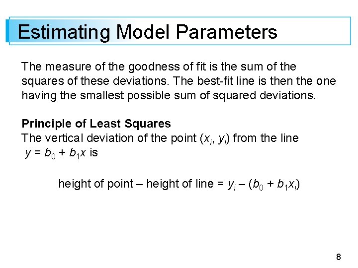
Estimating Model Parameters The measure of the goodness of fit is the sum of the squares of these deviations. The best-fit line is then the one having the smallest possible sum of squared deviations. Principle of Least Squares The vertical deviation of the point (xi, yi) from the line y = b 0 + b 1 x is height of point – height of line = yi – (b 0 + b 1 xi) 8

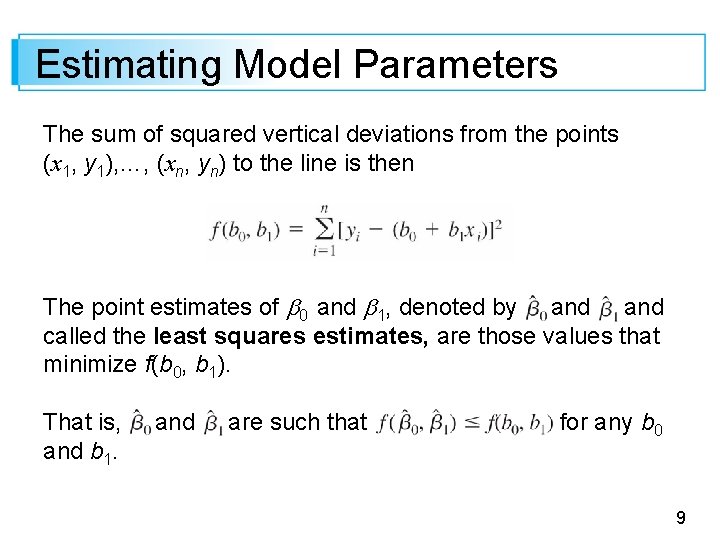
Estimating Model Parameters The sum of squared vertical deviations from the points (x 1, y 1), …, (xn, yn) to the line is then The point estimates of 0 and 1, denoted by and called the least squares estimates, are those values that minimize f(b 0, b 1). That is, and b 1. and are such that for any b 0 9

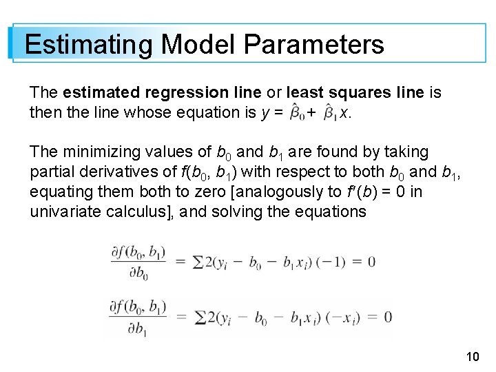
Estimating Model Parameters The estimated regression line or least squares line is then the line whose equation is y = + x. The minimizing values of b 0 and b 1 are found by taking partial derivatives of f(b 0, b 1) with respect to both b 0 and b 1, equating them both to zero [analogously to f (b) = 0 in univariate calculus], and solving the equations 10

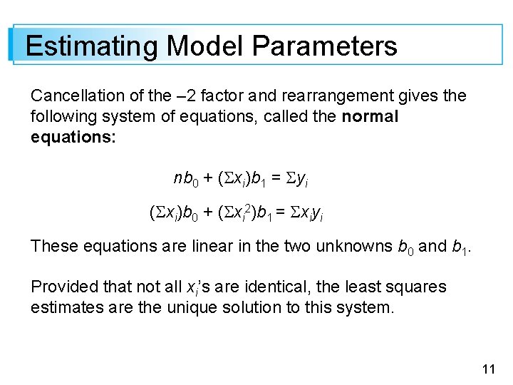
Estimating Model Parameters Cancellation of the – 2 factor and rearrangement gives the following system of equations, called the normal equations: nb 0 + ( xi)b 1 = yi ( xi)b 0 + ( xi 2)b 1 = xiyi These equations are linear in the two unknowns b 0 and b 1. Provided that not all xi’s are identical, the least squares estimates are the unique solution to this system. 11

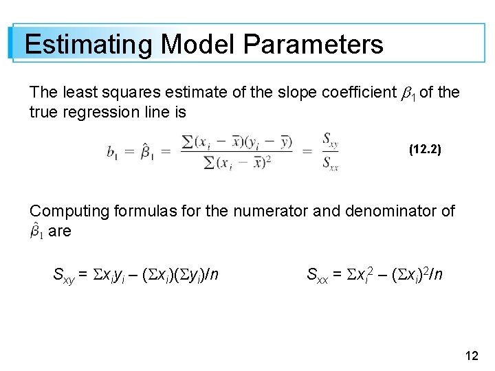
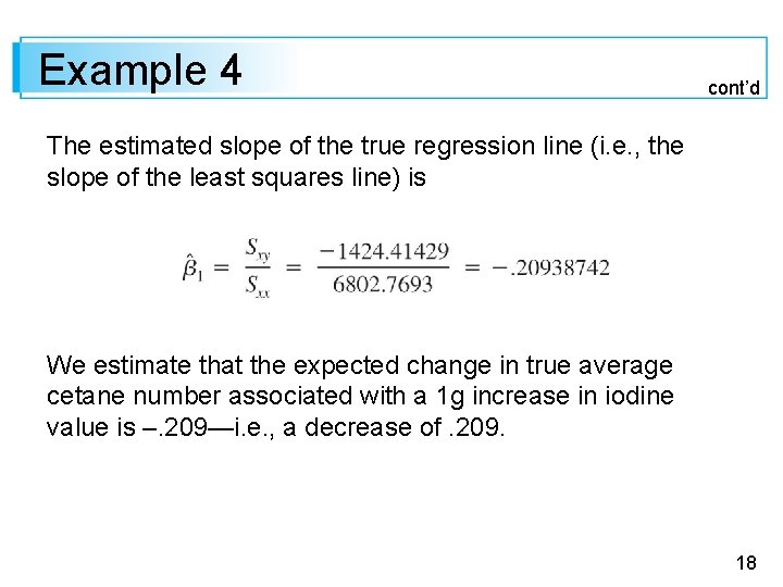
Estimating Model Parameters The least squares estimate of the slope coefficient 1 of the true regression line is (12. 2) Computing formulas for the numerator and denominator of are Sxy = xiyi – ( xi)( yi)/n Sxx = xi 2 – ( xi)2/n 12

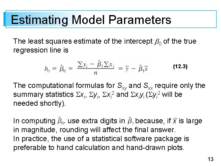
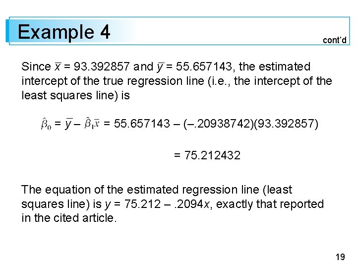
Estimating Model Parameters The least squares estimate of the intercept 0 of the true regression line is (12. 3) The computational formulas for Sxy and Sxx require only the summary statistics xi, yi, xi 2 and xiyi ( yi 2 will be needed shortly). In computing use extra digits in because, if x is large in magnitude, rounding will affect the final answer. In practice, the use of a statistical software package is preferable to hand calculation and hand-drawn plots. 13

Estimating Model Parameters Once again, be sure that the scatter plot shows a linear pattern with relatively homogenous variation before fitting the simple linear regression model. 14

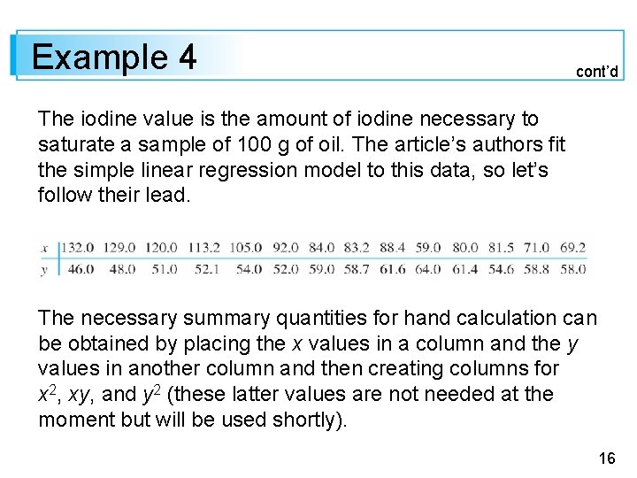
Example 4 The cetane number is a critical property in specifying the ignition quality of a fuel used in a diesel engine. Determination of this number for a biodiesel fuel is expensive and time-consuming. The article “Relating the Cetane Number of Biodiesel Fuels to Their Fatty Acid Composition: A Critical Study” (J. of Automobile Engr. , 2009: 565– 583) included the following data on x = iodine value (g) and y = cetane number for a sample of 14 biofuels. 15

Example 4 cont’d The iodine value is the amount of iodine necessary to saturate a sample of 100 g of oil. The article’s authors fit the simple linear regression model to this data, so let’s follow their lead. The necessary summary quantities for hand calculation can be obtained by placing the x values in a column and the y values in another column and then creating columns for x 2, xy, and y 2 (these latter values are not needed at the moment but will be used shortly). 16

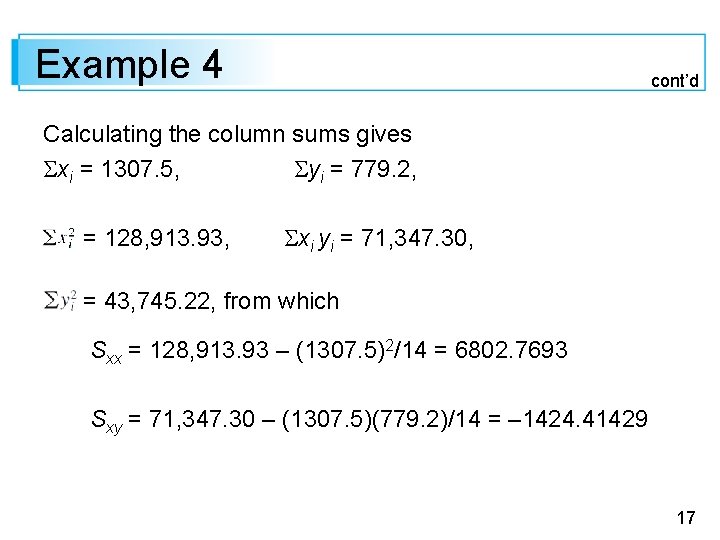
Example 4 cont’d Calculating the column sums gives xi = 1307. 5, yi = 779. 2, = 128, 913. 93, xi yi = 71, 347. 30, = 43, 745. 22, from which Sxx = 128, 913. 93 – (1307. 5)2/14 = 6802. 7693 Sxy = 71, 347. 30 – (1307. 5)(779. 2)/14 = – 1424. 41429 17

Example 4 cont’d The estimated slope of the true regression line (i. e. , the slope of the least squares line) is We estimate that the expected change in true average cetane number associated with a 1 g increase in iodine value is –. 209—i. e. , a decrease of. 209. 18

Example 4 cont’d Since x = 93. 392857 and y = 55. 657143, the estimated intercept of the true regression line (i. e. , the intercept of the least squares line) is =y– = 55. 657143 – (–. 20938742)(93. 392857) = 75. 212432 The equation of the estimated regression line (least squares line) is y = 75. 212 –. 2094 x, exactly that reported in the cited article. 19

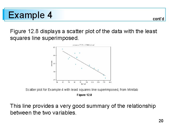
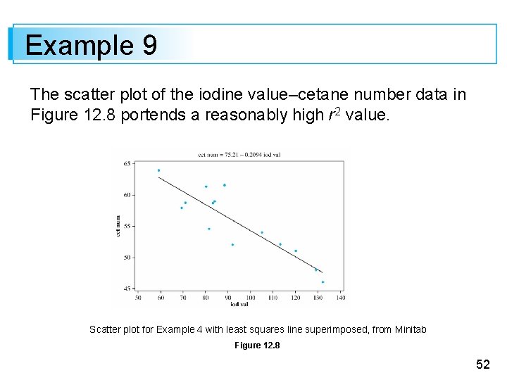
Example 4 cont’d Figure 12. 8 displays a scatter plot of the data with the least squares line superimposed. Scatter plot for Example 4 with least squares line superimposed, from Minitab Figure 12. 8 This line provides a very good summary of the relationship between the two variables. 20

Estimating 2 and 21

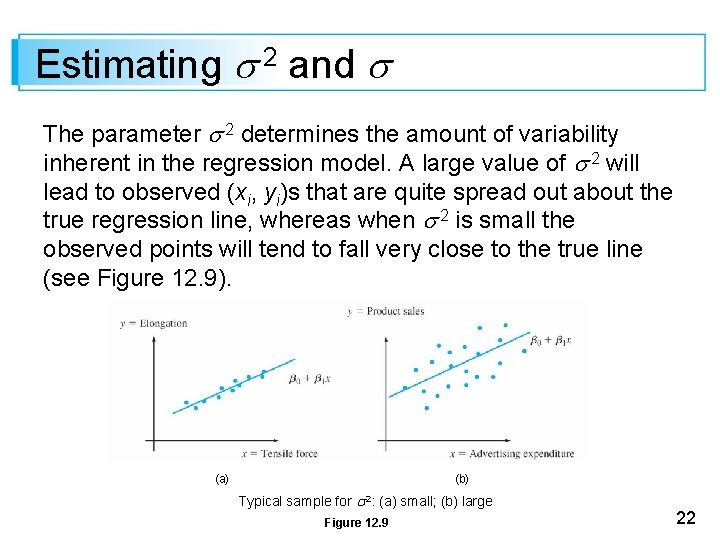
Estimating 2 and The parameter 2 determines the amount of variability inherent in the regression model. A large value of 2 will lead to observed (xi, yi)s that are quite spread out about the true regression line, whereas when 2 is small the observed points will tend to fall very close to the true line (see Figure 12. 9). (a) (b) Typical sample for 2: (a) small; (b) large Figure 12. 9 22

Estimating 2 and An estimate of 2 will be used in confidence interval (CI) formulas and hypothesis-testing procedures presented in the next two sections. Because the equation of the true line is unknown, the estimate is based on the extent to which the sample observations deviate from the estimated line. Many large deviations (residuals) suggest a large value of 2, whereas deviations all of which are small in magnitude suggest that 2 is small. 23

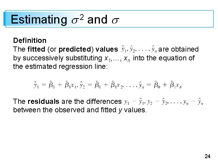
Estimating 2 and Definition The fitted (or predicted) values are obtained by successively substituting x 1, …, xn into the equation of the estimated regression line: The residuals are the differences between the observed and fitted y values. 24

Estimating 2 and In words, the predicted value is the value of y that we would predict or expect when using the estimated regression line with x = xi; is the height of the estimated regression line above the value xi for which the ith observation was made. The residual is the vertical deviation between the point (xi, yi) and the least squares line—a positive number if the point lies above the line and a negative number if it lies below the line. 25

Estimating 2 and If the residuals are all small in magnitude, then much of the variability in observed y values appears to be due to the linear relationship between x and y, whereas many large residuals suggest quite a bit of inherent variability in y relative to the amount due to the linear relation. 26

Estimating 2 and Assuming that the line in Figure 12. 7 is the least squares line, the residuals are identified by the vertical line segments from the observed points to the line. Deviations of observed data from line y = b 0 + b 1 x Figure 12. 7 27

Estimating 2 and When the estimated regression line is obtained via the principle of least squares, the sum of the residuals should in theory be zero. In practice, the sum may deviate a bit from zero due to rounding. 28

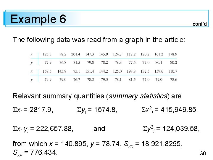
Example 6 Japan’s high population density has resulted in a multitude of resource-usage problems. One especially serious difficulty concerns waste removal. The article “Innovative Sludge Handling Through Pelletization Thickening” (Water Research, 1999: 3245– 3252) reported the development of a new compression machine for processing sewage sludge. An important part of the investigation involved relating the moisture content of compressed pellets (y, in %) to the machine’s filtration rate (x, in kg-DS/m/hr). 29

Example 6 cont’d The following data was read from a graph in the article: Relevant summary quantities (summary statistics) are xi = 2817. 9, xi yi = 222, 657. 88, yi = 1574. 8, x 2 i = 415, 949. 85, and y 2 i = 124, 039. 58, from which x = 140. 895, y = 78. 74, Sxx = 18, 921. 8295, Sxy = 776. 434. 30

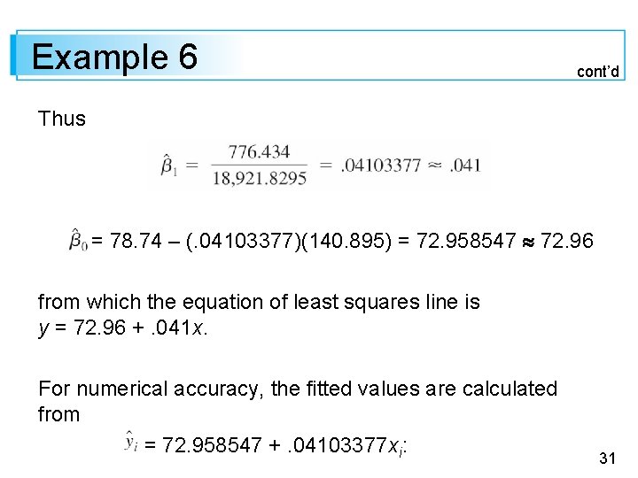
Example 6 cont’d Thus = 78. 74 – (. 04103377)(140. 895) = 72. 958547 72. 96 from which the equation of least squares line is y = 72. 96 +. 041 x. For numerical accuracy, the fitted values are calculated from = 72. 958547 +. 04103377 xi: 31

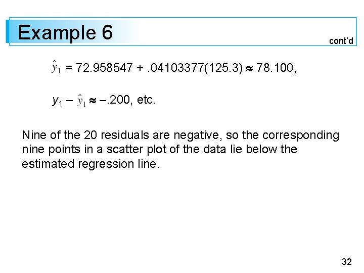
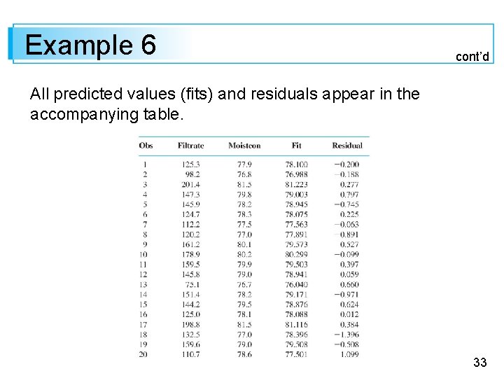
Example 6 cont’d = 72. 958547 +. 04103377(125. 3) 78. 100, y 1 – –. 200, etc. Nine of the 20 residuals are negative, so the corresponding nine points in a scatter plot of the data lie below the estimated regression line. 32

Example 6 cont’d All predicted values (fits) and residuals appear in the accompanying table. 33

Estimating 2 and In much the same way that the deviations from the mean in a one-sample situation were combined to obtain the estimate s 2 = (xi – x)2/(n – 1), the estimate of 2 in regression analysis is based on squaring and summing the residuals. We will continue to use the symbol s 2 for this estimated variance, so don’t confuse it with our previous s 2. 34

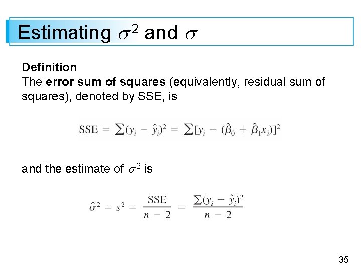
Estimating 2 and Definition The error sum of squares (equivalently, residual sum of squares), denoted by SSE, is and the estimate of 2 is 35

Estimating 2 and The divisor n – 2 in s 2 is the number of degrees of freedom (df) associated with SSE and the estimate s 2. This is because to obtain s 2, the two parameters 0 and 1 must first be estimated, which results in a loss of 2 df (just as had to be estimated in one sample problems, resulting in an estimated variance based on n – 1 df). Replacing each yi in the formula for s 2 by the rv Yi gives the estimator S 2. It can be shown that S 2 is an unbiased estimator for 2 (though the estimator S is not unbiased for ). 36

Estimating 2 and An interpretation of s here is similar to what we suggested earlier for the sample standard deviation: Very roughly, it is the size of a typical vertical deviation within the sample from the estimated regression line. 37

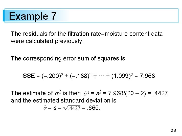
Example 7 The residuals for the filtration rate–moisture content data were calculated previously. The corresponding error sum of squares is SSE = (–. 200)2 + (–. 188)2 + ··· + (1. 099)2 = 7. 968 The estimate of 2 is then = s 2 = 7. 968/(20 – 2) =. 4427, and the estimated standard deviation is =s= =. 665. 38

Example 7 cont’d Roughly speaking, . 665 is the magnitude of a typical deviation from the estimated regression line—some points are closer to the line than this and others are further away. 39

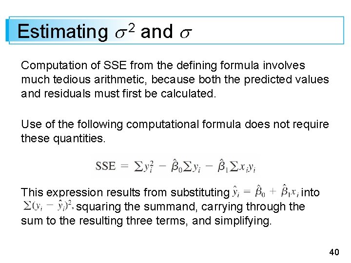
Estimating 2 and Computation of SSE from the defining formula involves much tedious arithmetic, because both the predicted values and residuals must first be calculated. Use of the following computational formula does not require these quantities. This expression results from substituting into squaring the summand, carrying through the sum to the resulting three terms, and simplifying. 40

Estimating 2 and This computational formula is especially sensitive to the effects of rounding in and so carrying as many digits as possible in intermediate computations will protect against round-off error. 41

The Coefficient of Determination 42

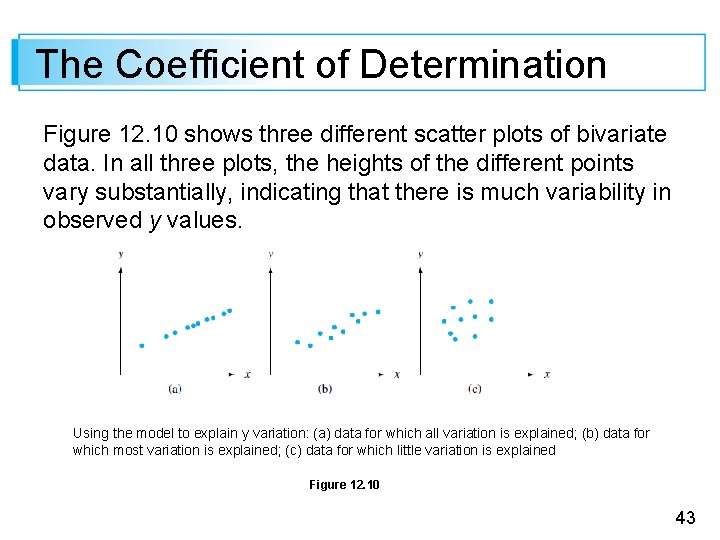
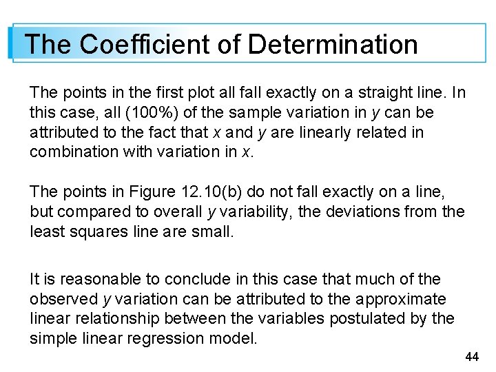
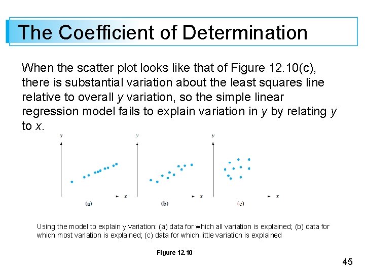
The Coefficient of Determination Figure 12. 10 shows three different scatter plots of bivariate data. In all three plots, the heights of the different points vary substantially, indicating that there is much variability in observed y values. Using the model to explain y variation: (a) data for which all variation is explained; (b) data for which most variation is explained; (c) data for which little variation is explained Figure 12. 10 43

The Coefficient of Determination The points in the first plot all fall exactly on a straight line. In this case, all (100%) of the sample variation in y can be attributed to the fact that x and y are linearly related in combination with variation in x. The points in Figure 12. 10(b) do not fall exactly on a line, but compared to overall y variability, the deviations from the least squares line are small. It is reasonable to conclude in this case that much of the observed y variation can be attributed to the approximate linear relationship between the variables postulated by the simple linear regression model. 44

The Coefficient of Determination When the scatter plot looks like that of Figure 12. 10(c), there is substantial variation about the least squares line relative to overall y variation, so the simple linear regression model fails to explain variation in y by relating y to x. Using the model to explain y variation: (a) data for which all variation is explained; (b) data for which most variation is explained; (c) data for which little variation is explained Figure 12. 10 45

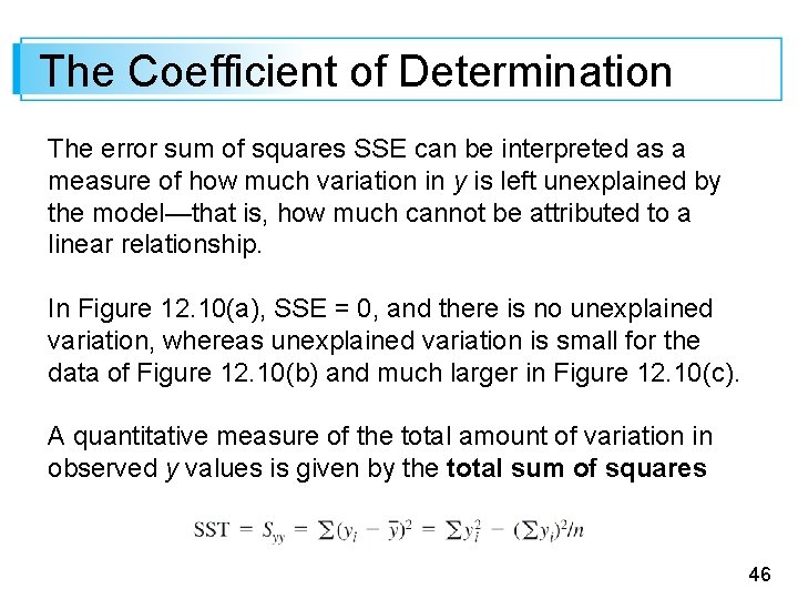
The Coefficient of Determination The error sum of squares SSE can be interpreted as a measure of how much variation in y is left unexplained by the model—that is, how much cannot be attributed to a linear relationship. In Figure 12. 10(a), SSE = 0, and there is no unexplained variation, whereas unexplained variation is small for the data of Figure 12. 10(b) and much larger in Figure 12. 10(c). A quantitative measure of the total amount of variation in observed y values is given by the total sum of squares 46

The Coefficient of Determination Total sum of squares is the sum of squared deviations about the sample mean of the observed y values. Thus the same number y is subtracted from each yi in SST, whereas SSE involves subtracting each different predicted value from the corresponding observed yi. 47

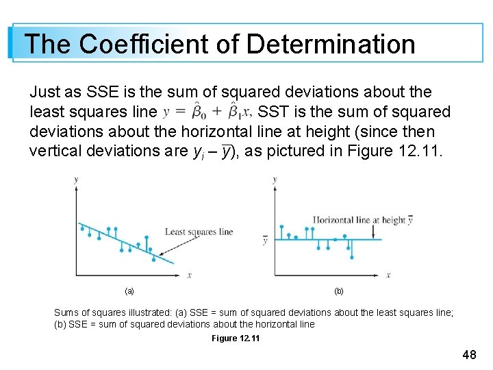
The Coefficient of Determination Just as SSE is the sum of squared deviations about the least squares line SST is the sum of squared deviations about the horizontal line at height (since then vertical deviations are yi – y), as pictured in Figure 12. 11. (a) (b) Sums of squares illustrated: (a) SSE = sum of squared deviations about the least squares line; (b) SSE = sum of squared deviations about the horizontal line Figure 12. 11 48

The Coefficient of Determination Furthermore, because the sum of squared deviations about the least squares line is smaller than the sum of squared deviations about any other line, SSE < SST unless the horizontal line itself is the least squares line. The ratio SSE/SST is the proportion of total variation that cannot be explained by the simple linear regression model, and 1 – SSE/SST (a number between 0 and 1) is the proportion of observed y variation explained by the model. 49

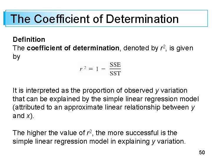
The Coefficient of Determination Definition The coefficient of determination, denoted by r 2, is given by It is interpreted as the proportion of observed y variation that can be explained by the simple linear regression model (attributed to an approximate linear relationship between y and x). The higher the value of r 2, the more successful is the simple linear regression model in explaining y variation. 50

The Coefficient of Determination When regression analysis is done by a statistical computer package, either r 2 or 100 r 2 (the percentage of variation explained by the model) is a prominent part of the output. If r 2 is small, an analyst will usually want to search for an alternative model (either a nonlinear model or a multiple regression model that involves more than a single independent variable) that can more effectively explain y variation. 51

Example 9 The scatter plot of the iodine value–cetane number data in Figure 12. 8 portends a reasonably high r 2 value. Scatter plot for Example 4 with least squares line superimposed, from Minitab Figure 12. 8 52

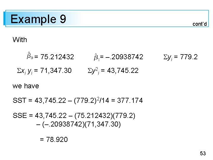
Example 9 cont’d With = 75. 212432 xi yi = 71, 347. 30 = –. 20938742 yi = 779. 2 y 2 i = 43, 745. 22 we have SST = 43, 745. 22 – (779. 2)2/14 = 377. 174 SSE = 43, 745. 22 – (75. 212432)(779. 2) – (–. 20938742)(71, 347. 30) = 78. 920 53

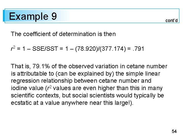
Example 9 cont’d The coefficient of determination is then r 2 = 1 – SSE/SST = 1 – (78. 920)/(377. 174) =. 791 That is, 79. 1% of the observed variation in cetane number is attributable to (can be explained by) the simple linear regression relationship between cetane number and iodine value (r 2 values are even higher than this in many scientific contexts, but social scientists would typically be ecstatic at a value anywhere near this large!). 54

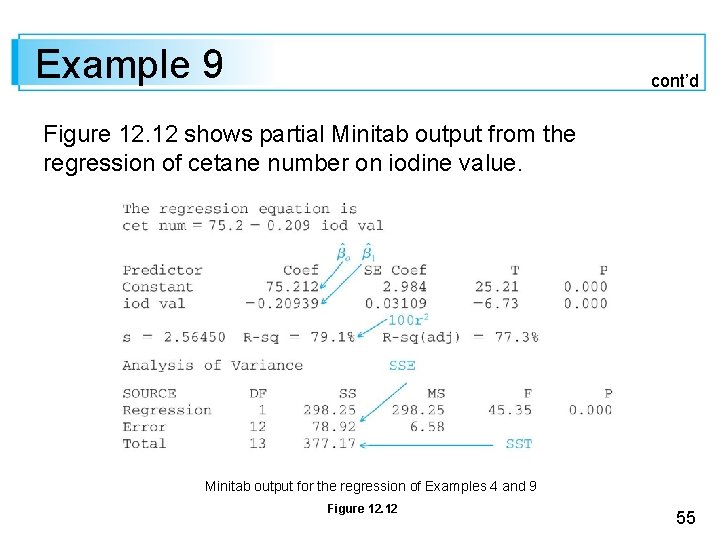
Example 9 cont’d Figure 12. 12 shows partial Minitab output from the regression of cetane number on iodine value. Minitab output for the regression of Examples 4 and 9 Figure 12. 12 55

Example 9 cont’d The software will also provide predicted values, residuals, and other information upon request. The formats used by other packages differ slightly from that of Minitab, but the information content is very similar. Regression sum of squares will be introduced shortly. 56

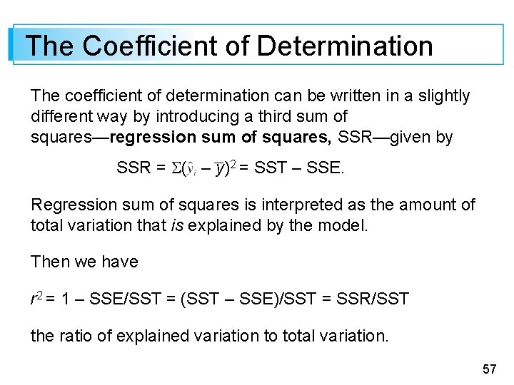
The Coefficient of Determination The coefficient of determination can be written in a slightly different way by introducing a third sum of squares—regression sum of squares, SSR—given by SSR = ( – y)2 = SST – SSE. Regression sum of squares is interpreted as the amount of total variation that is explained by the model. Then we have r 2 = 1 – SSE/SST = (SST – SSE)/SST = SSR/SST the ratio of explained variation to total variation. 57

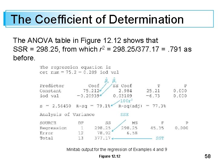
The Coefficient of Determination The ANOVA table in Figure 12. 12 shows that SSR = 298. 25, from which r 2 = 298. 25/377. 17 =. 791 as before. Minitab output for the regression of Examples 4 and 9 Figure 12. 12 58

Terminology and Scope of Regression Analysis 59

Terminology and Scope of Regression Analysis The term regression analysis was first used by Francis Galton in the late nineteenth century in connection with his work on the relationship between father’s height x and son’s height y. After collecting a number of pairs (xi, yi), Galton used the principle of least squares to obtain the equation of the estimated regression line, with the objective of using it to predict son’s height from father’s height. 60

Terminology and Scope of Regression Analysis In using the derived line, Galton found that if a father was above average in height, the son would also be expected to be above average in height, but not by as much as the father was. Similarly, the son of a shorter-than-average father would also be expected to be shorter than average, but not by as much as the father. Thus the predicted height of a son was “pulled back in” toward the mean; because regression means a coming or going back, Galton adopted the terminology regression line. 61

Terminology and Scope of Regression Analysis This phenomenon of being pulled back in toward the mean has been observed in many other situations (e. g. , batting averages from year to year in baseball) and is called the regression effect. Our discussion thus far has presumed that the independent variable is under the control of the investigator, so that only the dependent variable Y is random. This was not, however, the case with Galton’s experiment; fathers’ heights were not preselected, but instead both X and Y were random. 62

Terminology and Scope of Regression Analysis Methods and conclusions of regression analysis can be applied both when the values of the independent variable are fixed in advance and when they are random, but because the derivations and interpretations are more straightforward in the former case, we will continue to work explicitly with it. 63