12 Simple Linear Regression and Correlation Copyright Cengage

12 Simple Linear Regression and Correlation Copyright © Cengage Learning. All rights reserved.

12. 1 The Simple Linear Regression Model Copyright © Cengage Learning. All rights reserved.

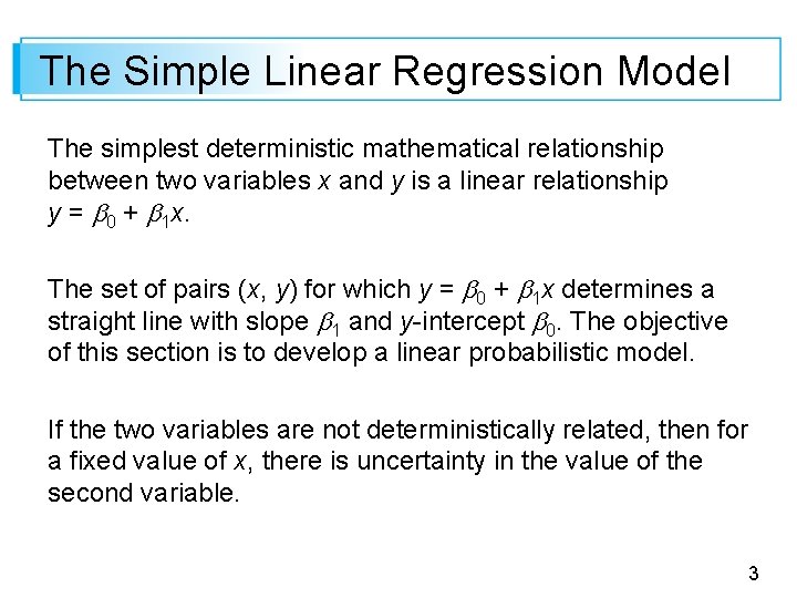
The Simple Linear Regression Model The simplest deterministic mathematical relationship between two variables x and y is a linear relationship y = 0 + 1 x. The set of pairs (x, y) for which y = 0 + 1 x determines a straight line with slope 1 and y-intercept 0. The objective of this section is to develop a linear probabilistic model. If the two variables are not deterministically related, then for a fixed value of x, there is uncertainty in the value of the second variable. 3

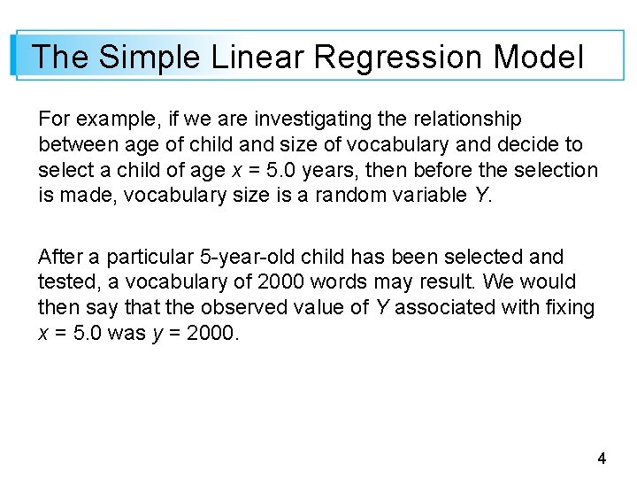
The Simple Linear Regression Model For example, if we are investigating the relationship between age of child and size of vocabulary and decide to select a child of age x = 5. 0 years, then before the selection is made, vocabulary size is a random variable Y. After a particular 5 -year-old child has been selected and tested, a vocabulary of 2000 words may result. We would then say that the observed value of Y associated with fixing x = 5. 0 was y = 2000. 4

The Simple Linear Regression Model More generally, the variable whose value is fixed by the experimenter will be denoted by x and will be called the independent, predictor, or explanatory variable. For fixed x, the second variable will be random; we denote this random variable and its observed value by Y and y, respectively, and refer to it as the dependent or response variable. Usually observations will be made for a number of settings of the independent variable. 5

The Simple Linear Regression Model Let x 1, x 2, …, xn denote values of the independent variable for which observations are made, and let Yi and yi, respectively, denote the random variable and observed value associated with xi. The available bivariate data then consists of the n pairs (x 1, y 1), (x 2, y 2), …, (xn, yn). A picture of this data called a scatter plot gives preliminary impressions about the nature of any relationship. In such a plot, each (xi, yi) is represented as a point plotted on a two dimensional coordinate system. 6

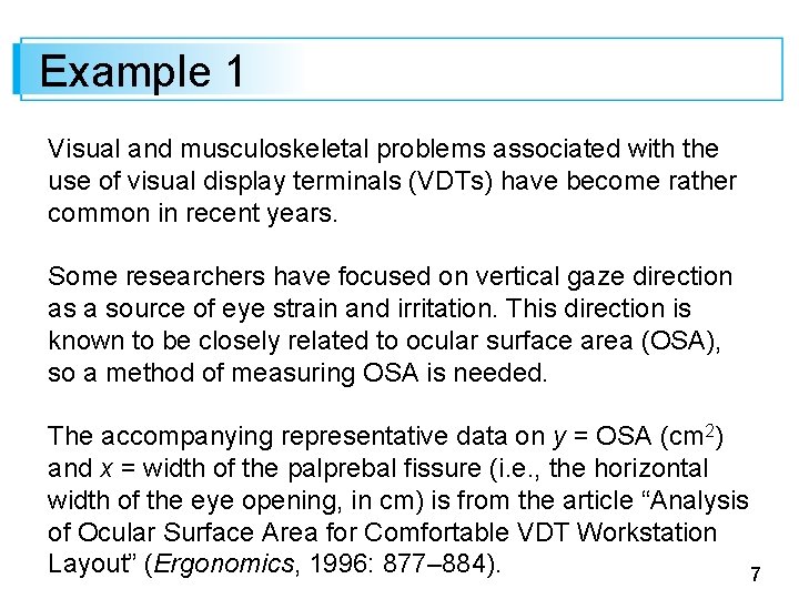
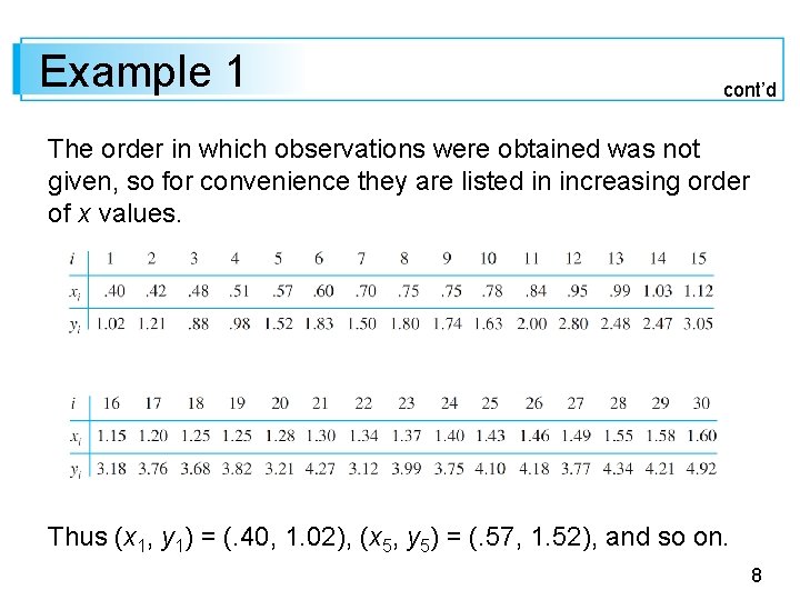
Example 1 Visual and musculoskeletal problems associated with the use of visual display terminals (VDTs) have become rather common in recent years. Some researchers have focused on vertical gaze direction as a source of eye strain and irritation. This direction is known to be closely related to ocular surface area (OSA), so a method of measuring OSA is needed. The accompanying representative data on y = OSA (cm 2) and x = width of the palprebal fissure (i. e. , the horizontal width of the eye opening, in cm) is from the article “Analysis of Ocular Surface Area for Comfortable VDT Workstation Layout” (Ergonomics, 1996: 877– 884). 7

Example 1 cont’d The order in which observations were obtained was not given, so for convenience they are listed in increasing order of x values. Thus (x 1, y 1) = (. 40, 1. 02), (x 5, y 5) = (. 57, 1. 52), and so on. 8

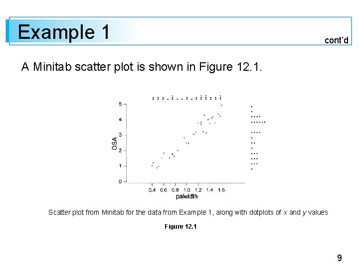
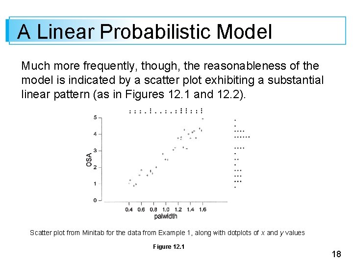
Example 1 cont’d A Minitab scatter plot is shown in Figure 12. 1. Scatter plot from Minitab for the data from Example 1, along with dotplots of x and y values Figure 12. 1 9

Example 1 cont’d We used an option that produced a dotplot of both the x values and y values individually along the right and top margins of the plot, which makes it easier to visualize the distributions of the individual variables (histograms or boxplots are alternative options). Here are some things to notice about the data and plot: • Several observations have identical x values yet different y values (e. g. x 8 = x 9 =. 75, but y 8 = 1. 80 and y 9 = 1. 74). Thus the value of y is not determined solely by x but also by various other factors. 10

Example 1 cont’d • There is a strong tendency for y to increase as x increases. That is, larger values of OSA tend to be associated with larger values of fissure width—a positive relationship between the variables. • It appears that the value of y could be predicted from x by finding a line that is reasonably close to the points in the plot (the authors of the cited article superimposed such a line on their plot). In other words, there is evidence of a substantial (though not perfect) linear relationship between the two variables. 11

A Linear Probabilistic Model 12

A Linear Probabilistic Model For the deterministic model y = 0 + 1 x, the actual observed value of y is a linear function of x. The appropriate generalization of this to a probabilistic model assumes that the expected value of Y is a linear function of x, but that for fixed x the variable. Y differs from its expected value by a random amount. 13

A Linear Probabilistic Model Definition The Simple Linear Regression Model There are parameters 0, 1, and 2, such that for any fixed value of the independent variable x, the dependent variable is a random variable related to x through the model equation (12. 1) Y = 0 + 1 x + The quantity in the model equation is a random variable, assumed to be normally distributed with E( ) = 0 and V( ) = 2. 14

A Linear Probabilistic Model The variable is usually referred to as the random deviation or random error term in the model. Without , any observed pair (x, y) would correspond to a point falling exactly on the line y = 0 + 1 x, called the true (or population) regression line. The inclusion of the random error term allows (x, y) to fall either above the true regression line (when > 0) or below the line (when < 0). 15

A Linear Probabilistic Model The points (x 1, y 1), …, (xn, yn) resulting from n independent observations will then be scattered about the true regression line, as illustrated in Figure 12. 3. Points corresponding to observations from the simple linear regression model Figure 12. 3 16

A Linear Probabilistic Model On occasion, the appropriateness of the simple linear regression model may be suggested by theoretical considerations (e. g. , there is an exact linear relationship between the two variables, with representing measurement error). 17

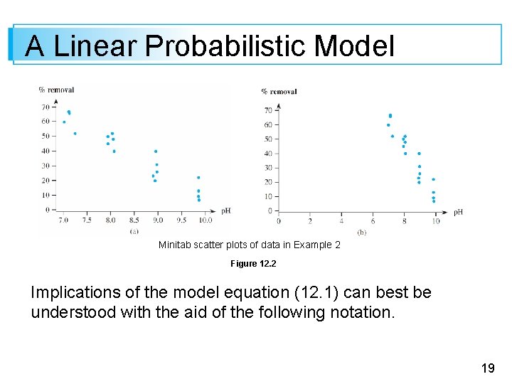
A Linear Probabilistic Model Much more frequently, though, the reasonableness of the model is indicated by a scatter plot exhibiting a substantial linear pattern (as in Figures 12. 1 and 12. 2). Scatter plot from Minitab for the data from Example 1, along with dotplots of x and y values Figure 12. 1 18

A Linear Probabilistic Model Minitab scatter plots of data in Example 2 Figure 12. 2 Implications of the model equation (12. 1) can best be understood with the aid of the following notation. 19

A Linear Probabilistic Model Let x denote a particular value of the independent variable x and Y x = the expected (or mean) value of Y when x has value x 2 Y x = the variance of Y when x has value x Alternative notation is E(Y | x ) and V(Y | x ). For example, if x = applied stress(kg/mm)2 and y = time-to-fracture (hr), then Y 20 would denote the expected value of time-to fracture when applied stress is 20 kg/mm 2. 20

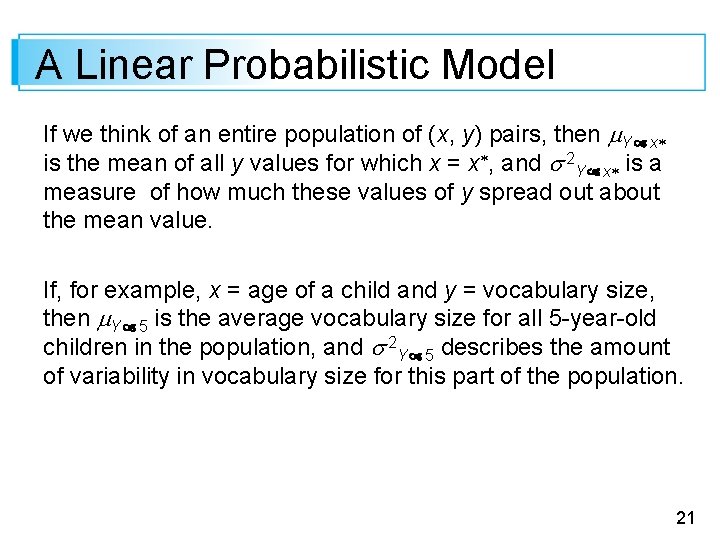
A Linear Probabilistic Model If we think of an entire population of (x, y) pairs, then Y x is the mean of all y values for which x = x , and 2 Y x is a measure of how much these values of y spread out about the mean value. If, for example, x = age of a child and y = vocabulary size, then Y 5 is the average vocabulary size for all 5 -year-old children in the population, and 2 Y 5 describes the amount of variability in vocabulary size for this part of the population. 21

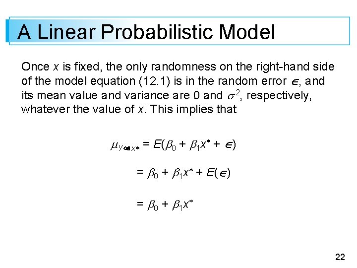
A Linear Probabilistic Model Once x is fixed, the only randomness on the right-hand side of the model equation (12. 1) is in the random error , and its mean value and variance are 0 and 2, respectively, whatever the value of x. This implies that Y x = E( 0 + 1 x + ) = 0 + 1 x + E( ) = 0 + 1 x 22

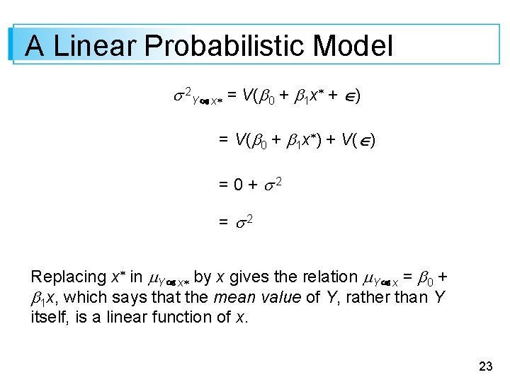
A Linear Probabilistic Model 2 Y x = V( 0 + 1 x + ) = V( 0 + 1 x ) + V( ) = 0 + 2 = 2 Replacing x in Y x by x gives the relation Y x = 0 + 1 x, which says that the mean value of Y, rather than Y itself, is a linear function of x. 23

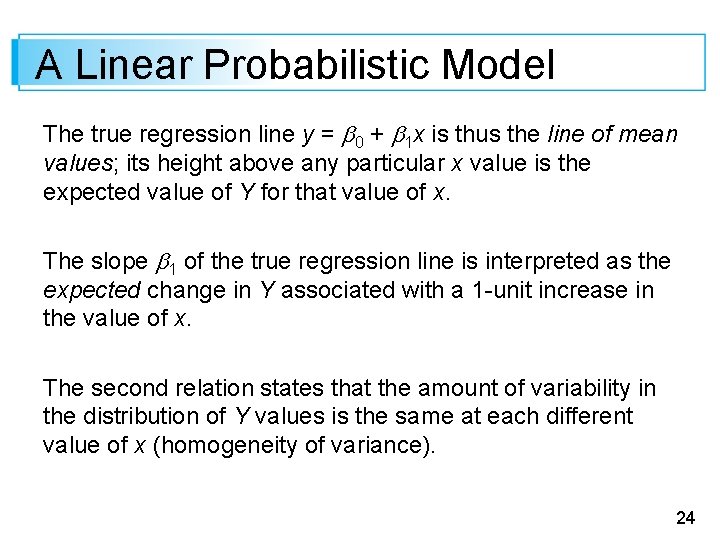
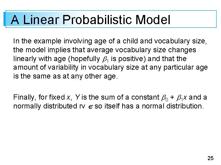
A Linear Probabilistic Model The true regression line y = 0 + 1 x is thus the line of mean values; its height above any particular x value is the expected value of Y for that value of x. The slope 1 of the true regression line is interpreted as the expected change in Y associated with a 1 -unit increase in the value of x. The second relation states that the amount of variability in the distribution of Y values is the same at each different value of x (homogeneity of variance). 24

A Linear Probabilistic Model In the example involving age of a child and vocabulary size, the model implies that average vocabulary size changes linearly with age (hopefully 1 is positive) and that the amount of variability in vocabulary size at any particular age is the same as at any other age. Finally, for fixed x, Y is the sum of a constant 0 + 1 x and a normally distributed rv so itself has a normal distribution. 25

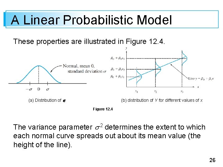
A Linear Probabilistic Model These properties are illustrated in Figure 12. 4. (a) Distribution of (b) distribution of Y for different values of x Figure 12. 4 The variance parameter 2 determines the extent to which each normal curve spreads out about its mean value (the height of the line). 26

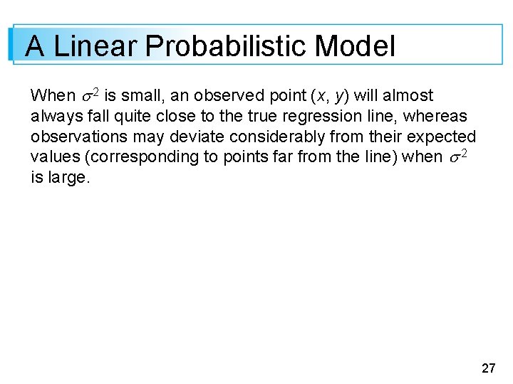
A Linear Probabilistic Model When 2 is small, an observed point (x, y) will almost always fall quite close to the true regression line, whereas observations may deviate considerably from their expected values (corresponding to points far from the line) when 2 is large. 27

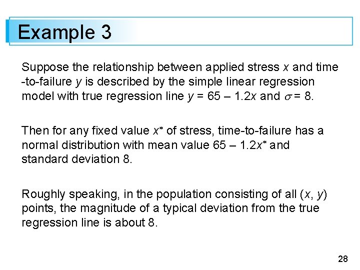
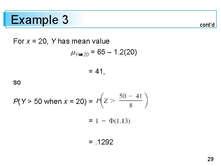
Example 3 Suppose the relationship between applied stress x and time -to-failure y is described by the simple linear regression model with true regression line y = 65 – 1. 2 x and = 8. Then for any fixed value x of stress, time-to-failure has a normal distribution with mean value 65 – 1. 2 x and standard deviation 8. Roughly speaking, in the population consisting of all (x, y) points, the magnitude of a typical deviation from the true regression line is about 8. 28

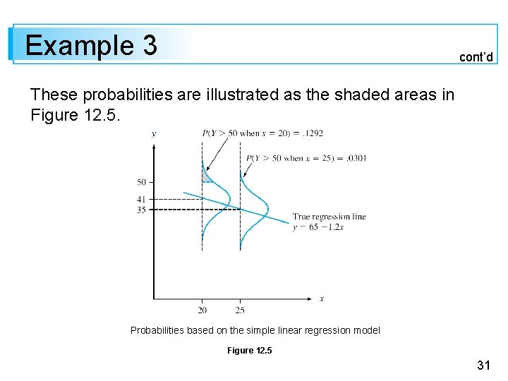
Example 3 cont’d For x = 20, Y has mean value Y 20 = 65 – 1. 2(20) = 41, so P(Y > 50 when x = 20) = = =. 1292 29

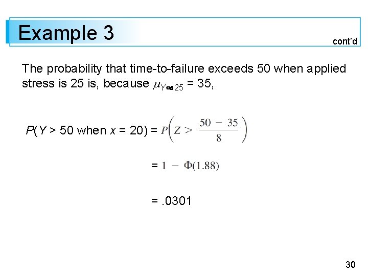
Example 3 cont’d The probability that time-to-failure exceeds 50 when applied stress is 25 is, because Y 25 = 35, P(Y > 50 when x = 20) = = =. 0301 30

Example 3 cont’d These probabilities are illustrated as the shaded areas in Figure 12. 5. Probabilities based on the simple linear regression model Figure 12. 5 31

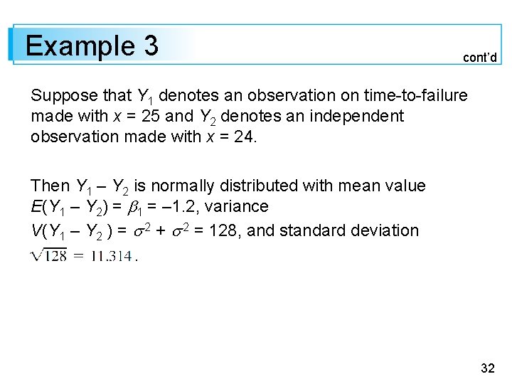
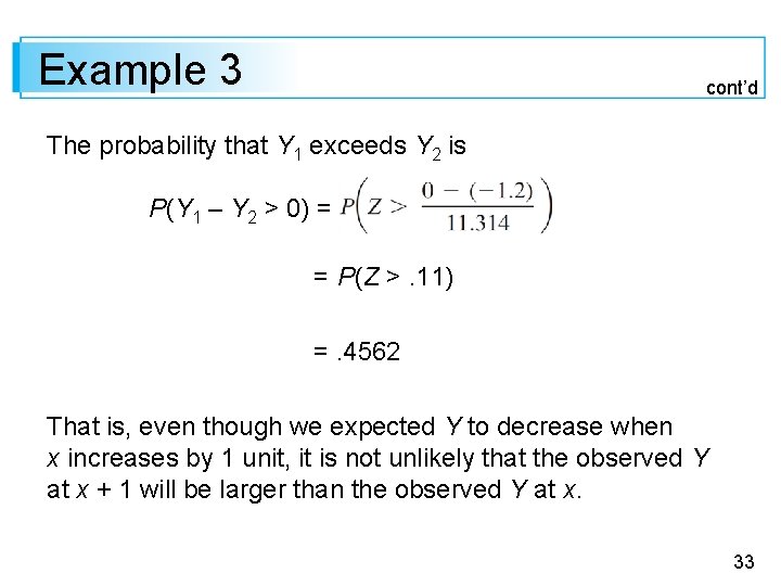
Example 3 cont’d Suppose that Y 1 denotes an observation on time-to-failure made with x = 25 and Y 2 denotes an independent observation made with x = 24. Then Y 1 – Y 2 is normally distributed with mean value E(Y 1 – Y 2) = 1 = – 1. 2, variance V(Y 1 – Y 2 ) = 2 + 2 = 128, and standard deviation. 32

Example 3 cont’d The probability that Y 1 exceeds Y 2 is P(Y 1 – Y 2 > 0) = = P(Z >. 11) =. 4562 That is, even though we expected Y to decrease when x increases by 1 unit, it is not unlikely that the observed Y at x + 1 will be larger than the observed Y at x. 33