Volatility Measurement Modeling and Forecasting Kafu Wong University

Volatility Measurement, Modeling, and Forecasting Ka-fu Wong University of Hong Kong 1

Importance of volatility n Good volatility forecasts are crucial for the implementation and evaluation of asset and derivative pricing theories as well as trading and hedging strategies. n Two assets: n an risky and a riskless (i. e. , volatility = 0) n Risky asset generally has a higher expected return than the riskless assets. n We would like to invest in a portfolio consisting of the two assets. n When the risky asset has a very high volatility, the portfolio will consist of the riskless asset only. n When the risky asset has a very low volatility, the portfolio will consist of more risky assets. 2

Importance of volatility n The variance of inflation may have impact on various macro and investment decisions. n High variance in inflation may also imply welfare loss. n Previous studies have tried to measure the time-varying variance of inflation. 3

Clustering of volatility n It is a well-established fact, dating back to Mandelbrot (1963) and Fama (1965), that financial returns display pronounced volatility clustering. n Therefore, models of volatility should allow such clustering. 4

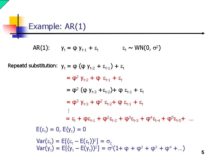
Example: AR(1): yt = φ yt-1 + et et ~ WN(0, s 2) Repeatd substitution: yt = φ (φ yt-2 + et-1) + et = φ2 yt-2 + φ et-1 + et = φ2 (φ yt-3 +et-2)+ φ et-1 + et = φ3 yt-3 + φ2 et-2+ φ et-1 + et … = et + φet-1 + φ2 et-2 + φ3 et-3 + φ4 et-4 + φ5 et-5+ … E(et) = 0, E(yt) = 0 Var(et) = E[(et – E(et))2] = s 2 Var(yt) = E[(yt – E(yt))2] = s 2(1+ φ + φ2 + φ3 + φ4 +…) 5

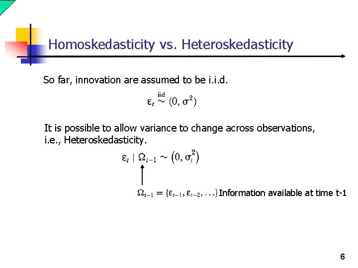
Homoskedasticity vs. Heteroskedasticity So far, innovation are assumed to be i. i. d. It is possible to allow variance to change across observations, i. e. , Heteroskedasticity. Information available at time t-1 6

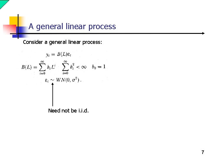
A general linear process Consider a general linear process: Need not be i. i. d. 7

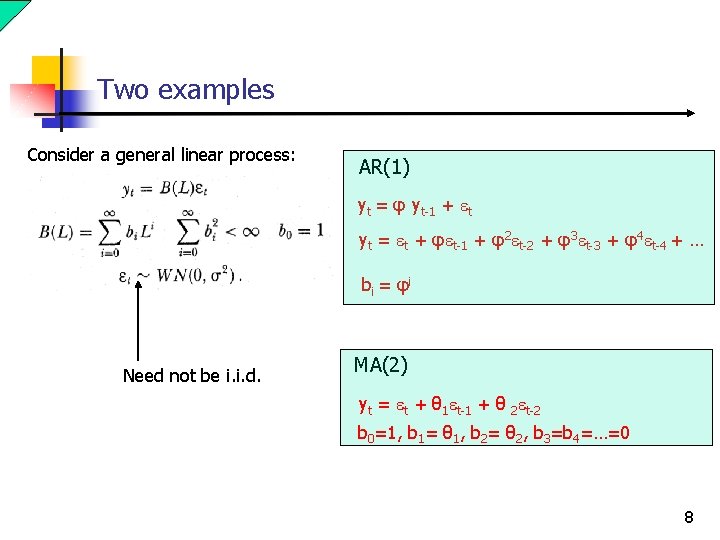
Two examples Consider a general linear process: AR(1) yt = φ yt-1 + et yt = et + φet-1 + φ2 et-2 + φ3 et-3 + φ4 et-4 + … b i = φi Need not be i. i. d. MA(2) yt = et + θ 1 et-1 + θ 2 et-2 b 0=1, b 1= θ 1, b 2= θ 2, b 3=b 4=…=0 8

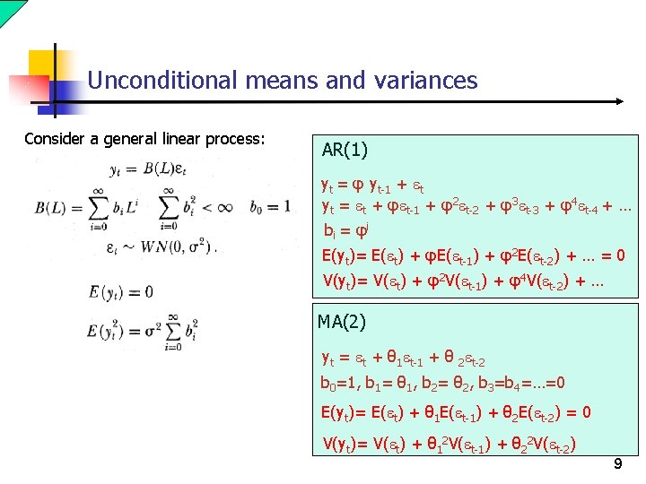
Unconditional means and variances Consider a general linear process: AR(1) yt = φ yt-1 + et yt = et + φet-1 + φ2 et-2 + φ3 et-3 + φ4 et-4 + … b i = φi E(yt)= E(et) + φE(et-1) + φ2 E(et-2) + … = 0 V(yt)= V(et) + φ2 V(et-1) + φ4 V(et-2) + … MA(2) yt = et + θ 1 et-1 + θ 2 et-2 b 0=1, b 1= θ 1, b 2= θ 2, b 3=b 4=…=0 E(yt)= E(et) + θ 1 E(et-1) + θ 2 E(et-2) = 0 V(yt)= V(et) + θ 12 V(et-1) + θ 22 V(et-2) 9

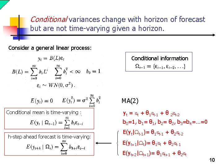
Conditional variances change with horizon of forecast but are not time-varying given a horizon. Consider a general linear process: Conditional information MA(2) Conditional mean is time-varying : yt = et + θ 1 et-1 + θ 2 et-2 b 0=1, b 1= θ 1, b 2= θ 2, b 3=b 4=…=0 h-step ahead forecast is time-varying: E(yt| t-1)= θ 1 et-1 + θ 2 et-2 E(yt+1| t)= θ 1 et + θ 2 et-1 E(yt+2| t+1)= θ 1 et+1 + θ 2 et 10

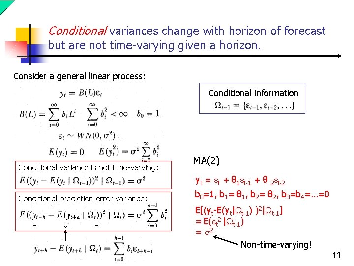
Conditional variances change with horizon of forecast but are not time-varying given a horizon. Consider a general linear process: Conditional information Conditional variance is not time-varying: MA(2) yt = et + θ 1 et-1 + θ 2 et-2 Conditional prediction error variance: b 0=1, b 1= θ 1, b 2= θ 2, b 3=b 4=…=0 E[(yt-E(yt| t-1) )2| t-1] = E(et 2 | t-1) = s 2 Non-time-varying! 11

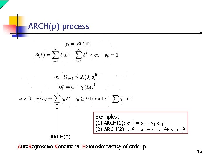
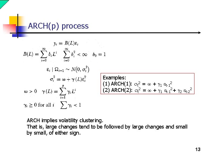
ARCH(p) process Examples: (1) ARCH(1): st 2 = w + g 1 et-12 (2) ARCH(2): st 2 = w + g 1 et-12+ g 2 et-22 ARCH(p) Auto. Regressive Conditional Heteroskedasticy of order p 12

ARCH(p) process Examples: (1) ARCH(1): st 2 = w + g 1 et-12 (2) ARCH(2): st 2 = w + g 1 et-12+ g 2 et-22 ARCH implies volatility clustering. That is, large changes tend to be followed by large changes and small by small, of either sign. 13

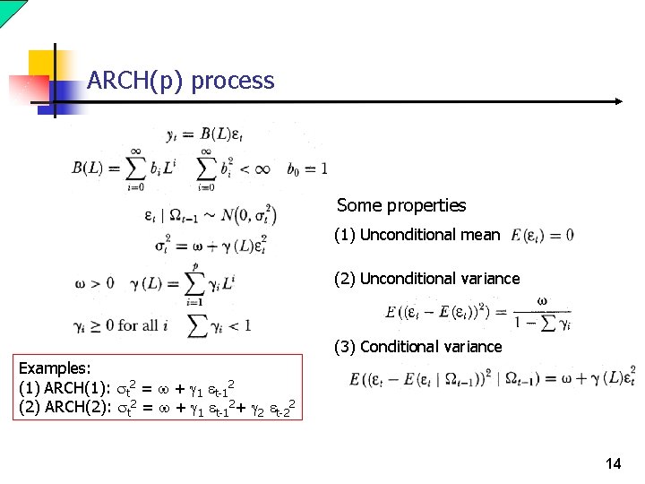
ARCH(p) process Some properties (1) Unconditional mean (2) Unconditional variance (3) Conditional variance Examples: (1) ARCH(1): st 2 = w + g 1 et-12 (2) ARCH(2): st 2 = w + g 1 et-12+ g 2 et-22 14

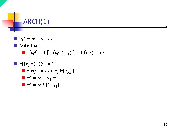
ARCH(1) n st 2 = w + g 1 et-12 n Note that n E[et 2] = E[ E(et 2| t-1) ] = E(st 2) = s 2 n E[(et-E(et))2] = ? n E[st 2] = w + g 1 E[et-12] n s 2 = w + g 1 s 2 n s 2 = w / (1 - g 1) 15

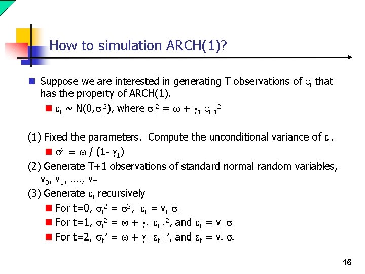
How to simulation ARCH(1)? n Suppose we are interested in generating T observations of et that has the property of ARCH(1). n et ~ N(0, st 2), where st 2 = w + g 1 et-12 (1) Fixed the parameters. Compute the unconditional variance of et. n s 2 = w / (1 - g 1) (2) Generate T+1 observations of standard normal random variables, v 0, v 1, …. , v. T (3) Generate et recursively n For t=0, st 2 = s 2, et = vt st n For t=1, st 2 = w + g 1 et-12, and et = vt st n For t=2, st 2 = w + g 1 et-12, and et = vt st 16

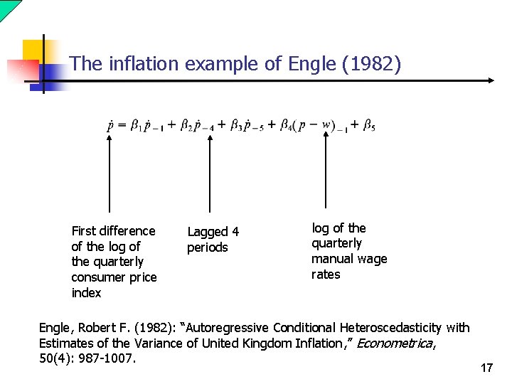
The inflation example of Engle (1982) First difference of the log of the quarterly consumer price index Lagged 4 periods log of the quarterly manual wage rates Engle, Robert F. (1982): “Autoregressive Conditional Heteroscedasticity with Estimates of the Variance of United Kingdom Inflation, ” Econometrica, 50(4): 987 -1007. 17

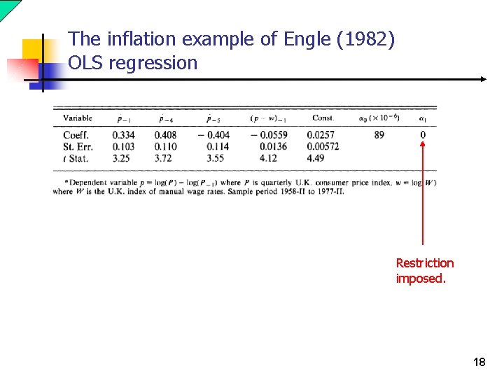
The inflation example of Engle (1982) OLS regression Restriction imposed. 18

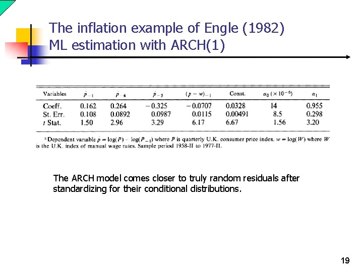
The inflation example of Engle (1982) ML estimation with ARCH(1) The ARCH model comes closer to truly random residuals after standardizing for their conditional distributions. 19

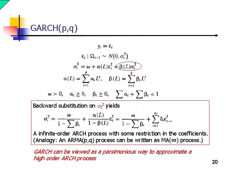
GARCH(p, q) Backward substitution on st 2 yields A infinite-order ARCH process with some restriction in the coefficients. (Analogy: An ARMA(p, q) process can be written as MA(∞) process. ) GARCH can be viewed as a parsimonious way to approximate a high order ARCH process 20

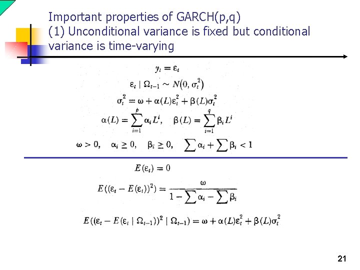
Important properties of GARCH(p, q) (1) Unconditional variance is fixed but conditional variance is time-varying 21

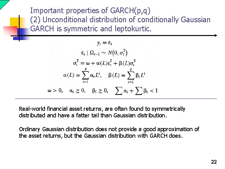
Important properties of GARCH(p, q) (2) Unconditional distribution of conditionally Gaussian GARCH is symmetric and leptokurtic. Real-world financial asset returns, are often found to symmetrically distributed and have a fatter tail than Gaussian distribution. Ordinary Gaussian distribution does not provide a good approximation of the asset returns, but the Gaussian distribution with GARCH does. 22

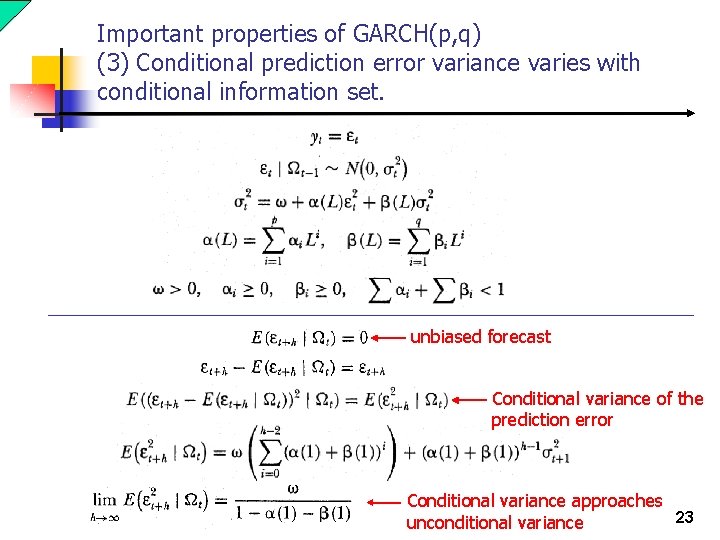
Important properties of GARCH(p, q) (3) Conditional prediction error variance varies with conditional information set. unbiased forecast Conditional variance of the prediction error Conditional variance approaches 23 unconditional variance

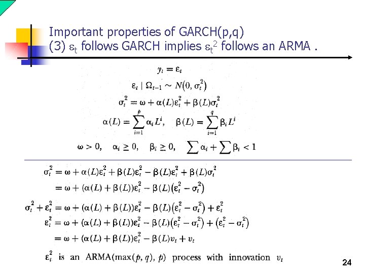
Important properties of GARCH(p, q) (3) et follows GARCH implies et 2 follows an ARMA. 24

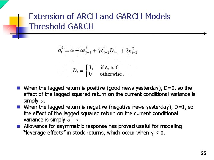
Extension of ARCH and GARCH Models Threshold GARCH n When the lagged return is positive (good news yesterday), D=0, so the effect of the lagged squared return on the current conditional variance is simply a. n When the lagged return is negative (negative news yesterday), D=1, so the effect of the lagged squared return on the current conditional variance is simply a + g. n Allowance for asymmetric response has proved useful for modeling “leverage effects” in stock returns, which occur when g < 0. 25

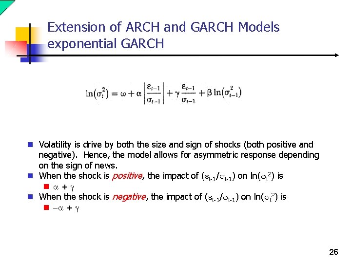
Extension of ARCH and GARCH Models exponential GARCH n Volatility is drive by both the size and sign of shocks (both positive and negative). Hence, the model allows for asymmetric response depending on the sign of news. n When the shock is positive, the impact of (et-1/st-1) on ln(st 2) is n a+g n When the shock is negative, the impact of (et-1/st-1) on ln(st 2) is n -a + g 26

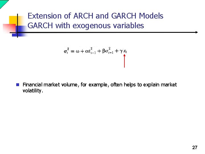
Extension of ARCH and GARCH Models GARCH with exogenous variables n Financial market volume, for example, often helps to explain market volatility. 27

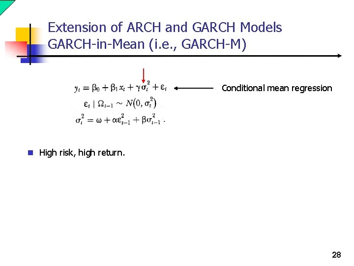
Extension of ARCH and GARCH Models GARCH-in-Mean (i. e. , GARCH-M) Conditional mean regression n High risk, high return. 28

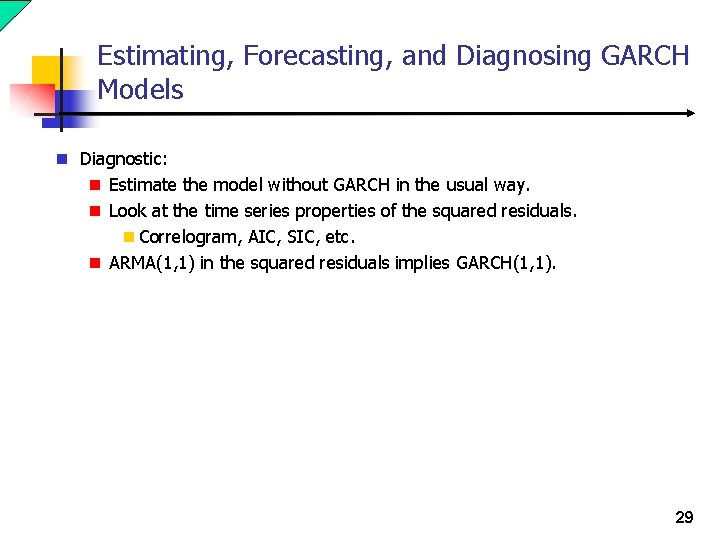
Estimating, Forecasting, and Diagnosing GARCH Models n Diagnostic: n Estimate the model without GARCH in the usual way. n Look at the time series properties of the squared residuals. n Correlogram, AIC, SIC, etc. n ARMA(1, 1) in the squared residuals implies GARCH(1, 1). 29

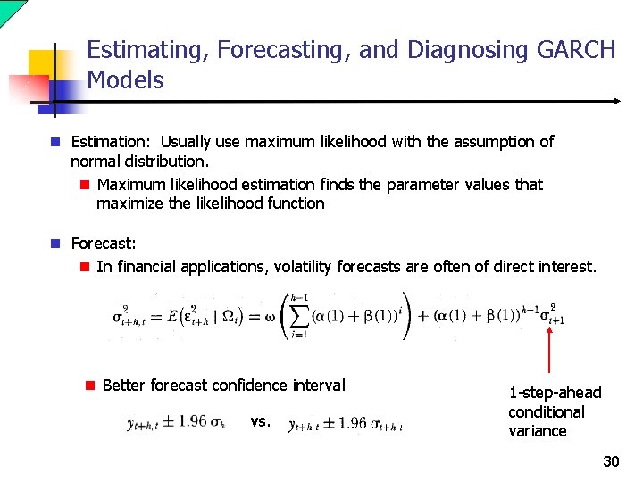
Estimating, Forecasting, and Diagnosing GARCH Models n Estimation: Usually use maximum likelihood with the assumption of normal distribution. n Maximum likelihood estimation finds the parameter values that maximize the likelihood function n Forecast: n In financial applications, volatility forecasts are often of direct interest. n Better forecast confidence interval vs. 1 -step-ahead conditional variance 30

Application: Stock Market Volatility n Objective: Model and forecast the volatility of daily returns on the New York Stock Exchange n Data: n Daily returns on the New York Stock Exchange (NYSE) form January 1, 1988, through December 31, 2001. n Excluding holidays, there are 3531 observations. n Estimation: 1 -3461 n Forecast: 3462 -3531. 31

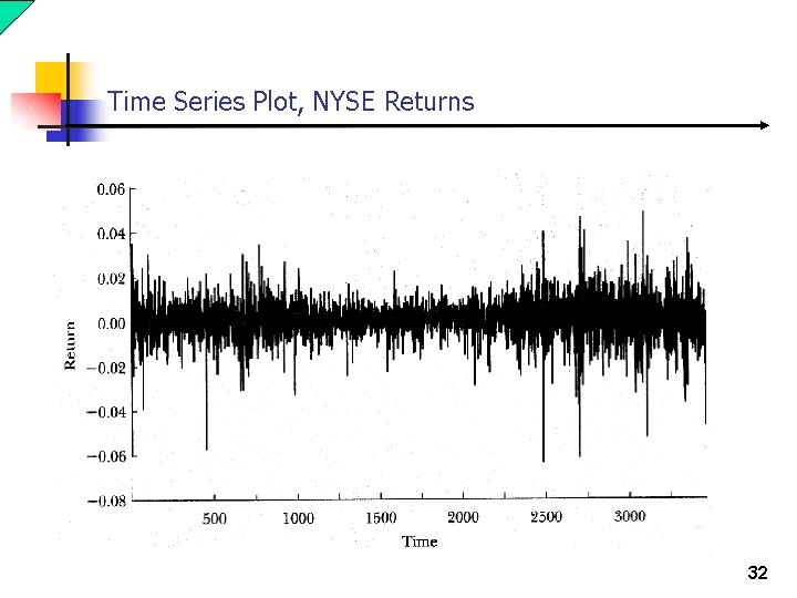
Time Series Plot, NYSE Returns 32

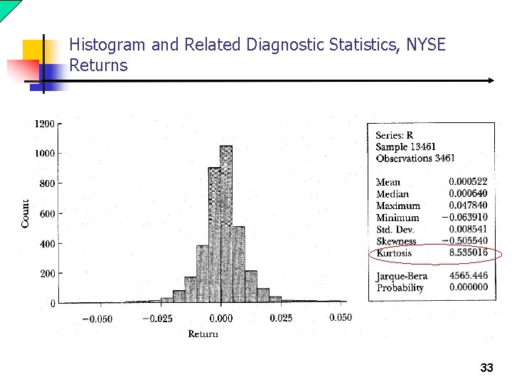
Histogram and Related Diagnostic Statistics, NYSE Returns 33

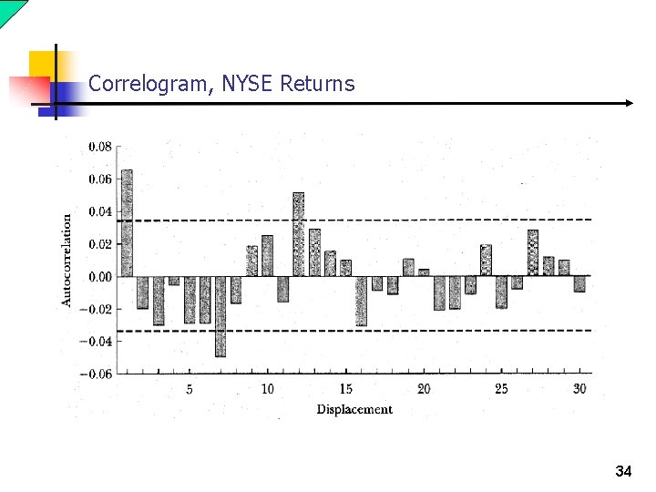
Correlogram, NYSE Returns 34

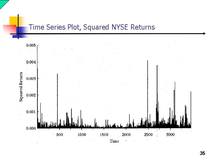
Time Series Plot, Squared NYSE Returns 35

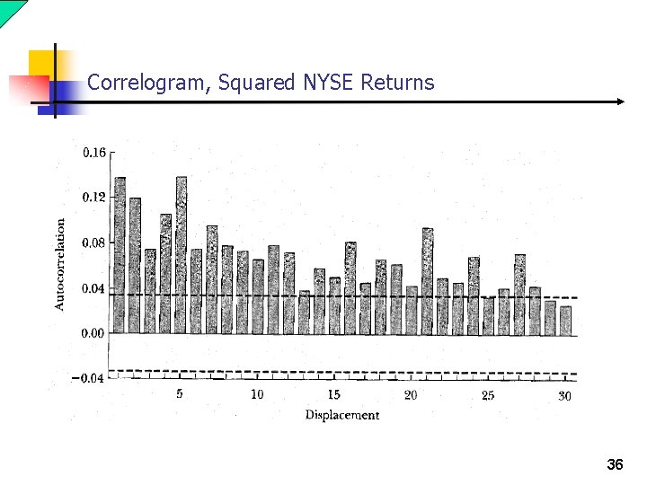
Correlogram, Squared NYSE Returns 36

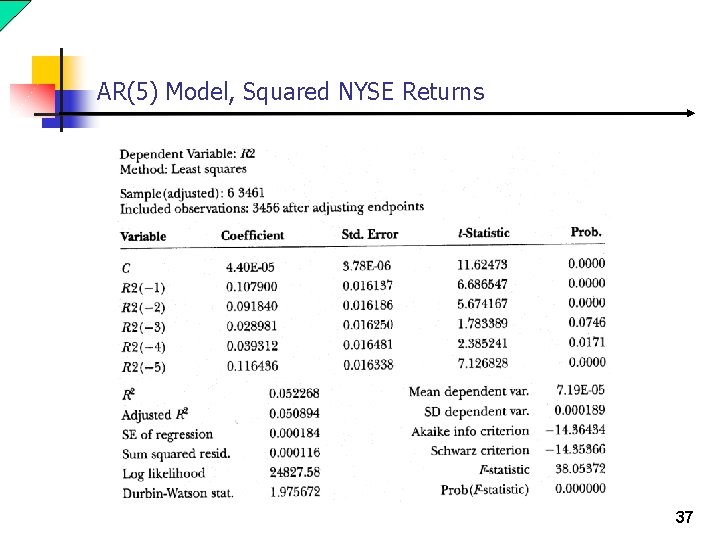
AR(5) Model, Squared NYSE Returns 37

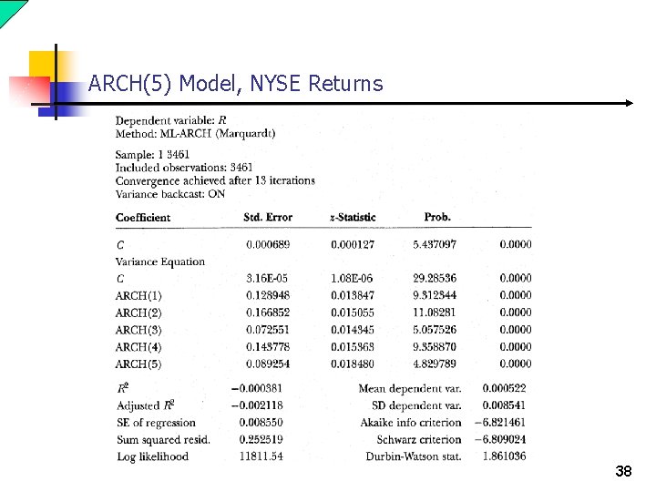
ARCH(5) Model, NYSE Returns 38

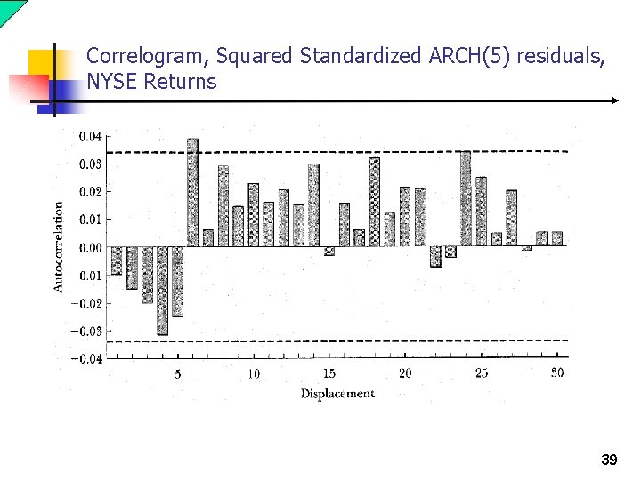
Correlogram, Squared Standardized ARCH(5) residuals, NYSE Returns 39

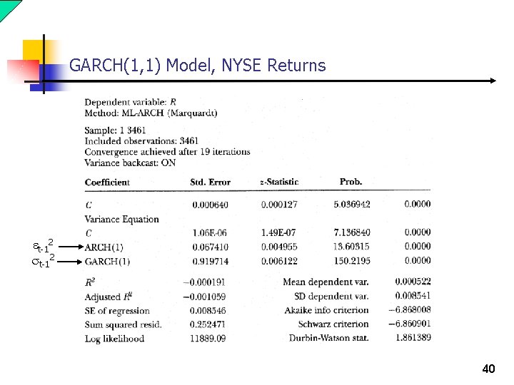
GARCH(1, 1) Model, NYSE Returns et-12 st-12 40

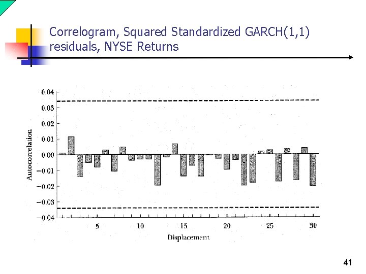
Correlogram, Squared Standardized GARCH(1, 1) residuals, NYSE Returns 41

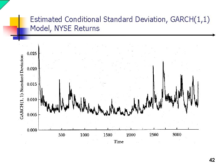
Estimated Conditional Standard Deviation, GARCH(1, 1) Model, NYSE Returns 42

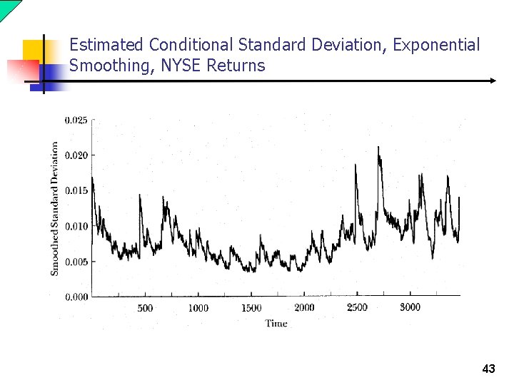
Estimated Conditional Standard Deviation, Exponential Smoothing, NYSE Returns 43

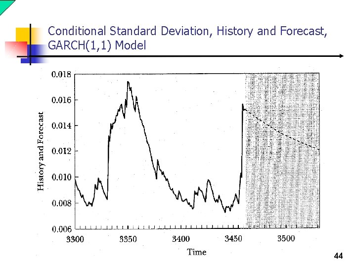
Conditional Standard Deviation, History and Forecast, GARCH(1, 1) Model 44

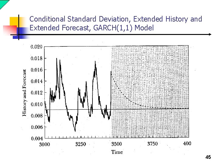
Conditional Standard Deviation, Extended History and Extended Forecast, GARCH(1, 1) Model 45

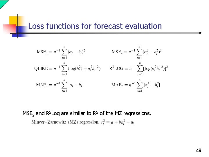
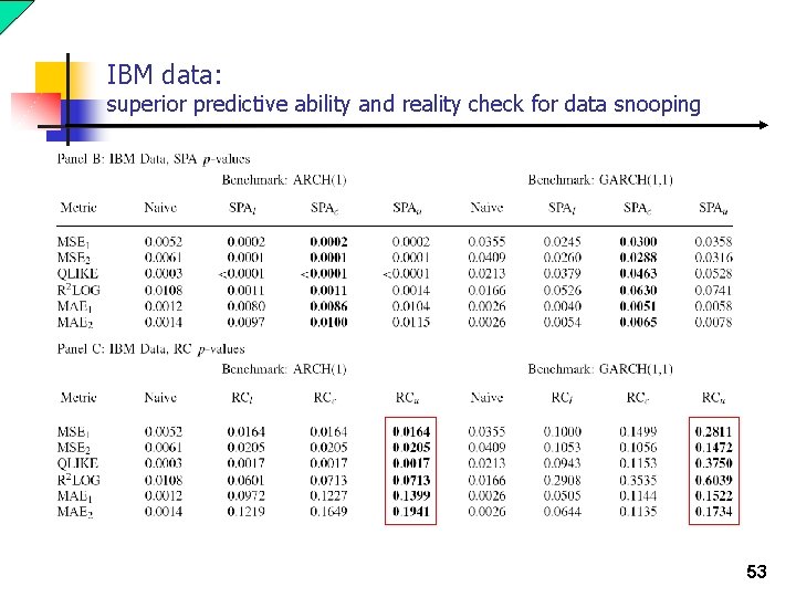
Is GARCH(1, 1) enough most of the time? n 330 GARCH-type models are compared in terms of their ability to forecast the one-day-ahead conditional variance. n The models are evaluated out-of-sample using six different loss functions, where the realized variance is substituted for the latent conditional variance. Hansen, Peter R. and Asger Lunde (2005): “A Forecast Comparison Of Volatility Models: Does Anything Beat A GARCH(1, 1)? ” Journal of Applied Econometrics, 20: 873 -889. 46

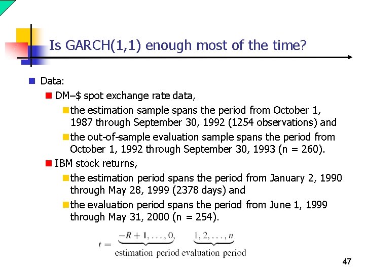
Is GARCH(1, 1) enough most of the time? n Data: n DM–$ spot exchange rate data, n the estimation sample spans the period from October 1, 1987 through September 30, 1992 (1254 observations) and n the out-of-sample evaluation sample spans the period from October 1, 1992 through September 30, 1993 (n = 260). n IBM stock returns, n the estimation period spans the period from January 2, 1990 through May 28, 1999 (2378 days) and n the evaluation period spans the period from June 1, 1999 through May 31, 2000 (n = 254). 47

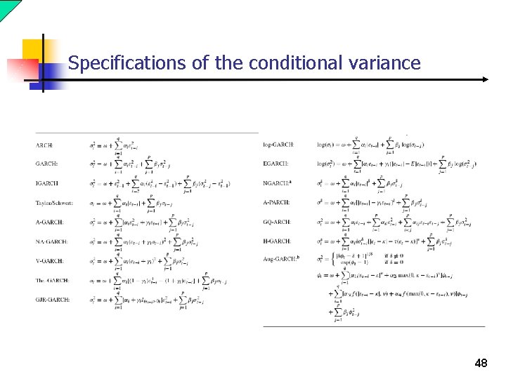
Specifications of the conditional variance 48

Loss functions forecast evaluation MSE 2 and R 2 Log are similar to R 2 of the MZ regressions. 49

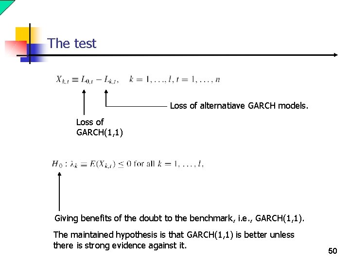
The test Loss of alternatiave GARCH models. Loss of GARCH(1, 1) Giving benefits of the doubt to the benchmark, i. e. , GARCH(1, 1). The maintained hypothesis is that GARCH(1, 1) is better unless there is strong evidence against it. 50

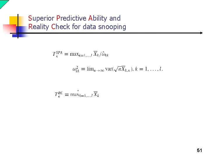
Superior Predictive Ability and Reality Check for data snooping 51

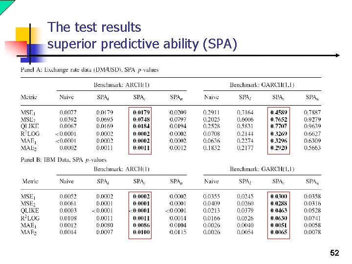
The test results superior predictive ability (SPA) 52

IBM data: superior predictive ability and reality check for data snooping 53

Does Anything Beat A GARCH(1, 1)? n No. So, use GARCH(1, 1) if no other information is available. 54

End 55