VOLATILITY ADJUSTMENT FULL AND WEIGHTED VOLATILITY ADJUSTMENT FOR

VOLATILITY ADJUSTMENT (FULL) AND WEIGHTED VOLATILITY ADJUSTMENT FOR THE BLACK SCHOLES MODEL Michael Aussieker Oliver Grace Fredrik Jonsӓll

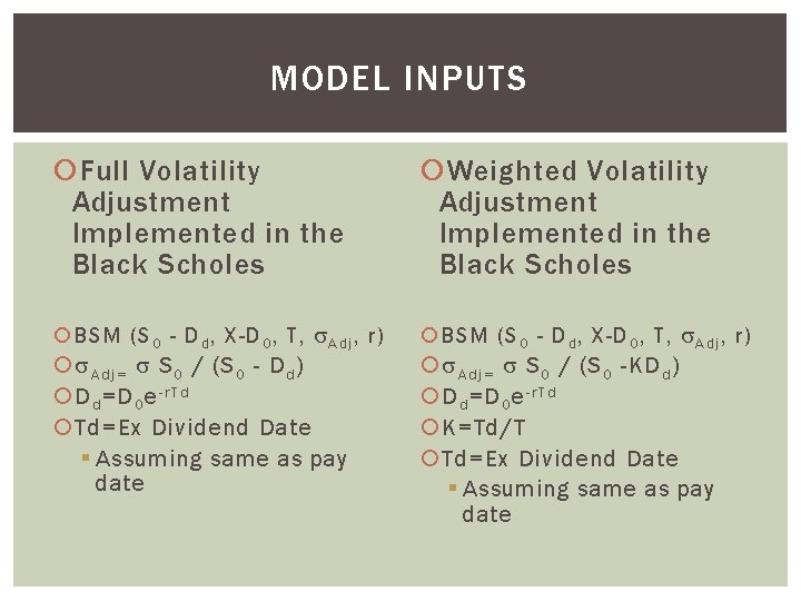
MODEL INPUTS Full Volatility Adjustment Implemented in the Black Scholes Weighted Volatility Adjustment Implemented in the Black Scholes BSM (S 0 - D d , X-D 0 , T, A d j , r) A d j = S 0 / (S 0 - D d ) D d =D 0 e - r T d Td=Ex Dividend Date § Assuming same as pay date BSM (S 0 - D d , X-D 0 , T, A d j , r) A d j = S 0 / (S 0 -KD d ) D d =D 0 e - r T d K=Td/T Td=Ex Dividend Date § Assuming same as pay date

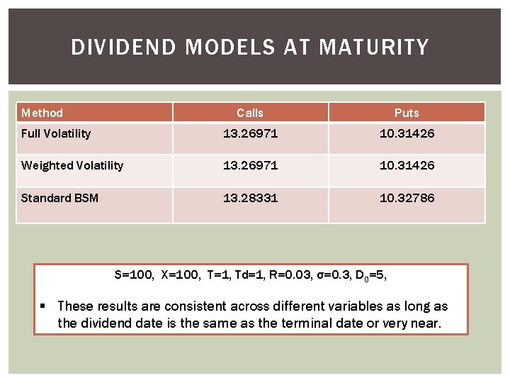
DIVIDEND MODELS AT MATURITY Method Calls Puts Full Volatility 13. 26971 10. 31426 Weighted Volatility 13. 26971 10. 31426 Standard BSM 13. 28331 10. 32786 S=100, X=100, T=1, Td=1, R=0. 03, σ=0. 3, D 0=5, § These results are consistent across different variables as long as the dividend date is the same as the terminal date or very near.

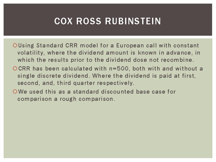
COX ROSS RUBINSTEIN Using Standard CRR model for a European call with constant volatility, where the dividend amount is known in advance, in which the results prior to the dividend dose not recombine. CRR has been calculated with n=500, both with and without a single discrete dividend. Where the dividend is paid at first, second, and, third quarter respectively. We used this as a standard discounted base case for comparison a rough comparison.

DIFFERENCE WITH BSM AT $2 DIV 0. 25 0. 2 FV. 25 0. 15 FV. 75 WV. 25 0. 1 WV. 5 WV. 75 CRR. 25 0. 05 CRR. 75 0 70 -0. 05 80 90 100 Strike 110 120

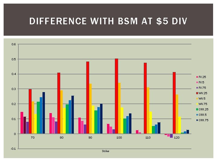
DIFFERENCE WITH BSM AT $5 DIV 0. 6 0. 5 0. 4 FV. 25 FV. 75 0. 3 WV. 25 WV. 5 0. 2 WV. 75 CRR. 25 CRR. 5 0. 1 CRR. 75 0 70 -0. 1 80 90 100 Strike 110 120

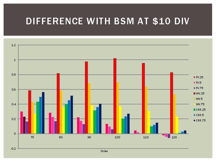
DIFFERENCE WITH BSM AT $10 DIV 1. 2 1 0. 8 FV. 25 FV. 75 0. 6 WV. 25 WV. 5 0. 4 WV. 75 CRR. 25 CRR. 5 0. 2 CRR. 75 0 70 -0. 2 80 90 100 Strike 110 120

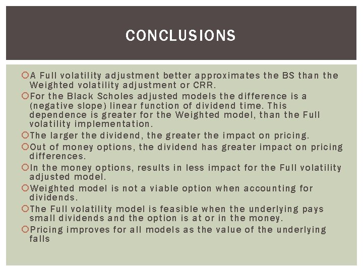
CONCLUSIONS A Full volatility adjustment better approximates the BS than the Weighted volatility adjustment or CRR. For the Black Scholes adjusted models the difference is a (negative slope) linear function of dividend time. This dependence is greater for the Weighted model, than the Full volatility implementation. The larger the dividend, the greater the impact on pricing. Out of money options, the dividend has greater impact on pricing differences. In the money options, results in less impact for the Full volatility adjusted model. Weighted model is not a viable option when accounting for dividends. The Full volatility model is feasible when the underlying pays small dividends and the option is at or in the money. Pricing improves for all models as the value of the underlying falls

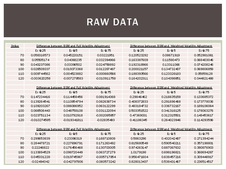
RAW DATA Strike 70 80 90 100 110 120 Difference between BSM and Full Volatility Adjustment Ex @. 25 Ex @. 75 0. 058316573 0. 045220151 0. 03221951 0. 05505174 0. 04368235 0. 032394966 0. 043237086 0. 03396502 0. 024758892 0. 026509337 0. 019373368 0. 012287487 0. 009744562 0. 004523882 -0. 000660566 -0. 003620258 -0. 007278583 -0. 010911758 Difference between BSM and Weighted Volatility Adjustment Ex @. 25 Ex @. 75 0. 120523292 0. 08671919 0. 052981061 0. 163387609 0. 11580473 0. 068403046 0. 192318966 0. 13311066 0. 074208246 0. 200021157 0. 134732407 0. 069806858 0. 188393566 0. 123328183 0. 05859128 0. 164202311 0. 104398851 0. 044821488 70 80 90 100 110 120 Difference between BSM and Full Volatility Adjustment Ex @. 25 Ex @. 75 0. 147234416 0. 114458456 0. 081914368 0. 139264541 0. 110854794 0. 082638734 0. 109203267 0. 086086952 0. 063122299 0. 066506443 0. 048758108 0. 031122094 0. 023751134 0. 010792918 -0. 002085857 -0. 010274585 -0. 019341811 -0. 02835493 Difference between BSM and Weighted Volatility Adjustment Ex @. 25 Ex @. 75 0. 29846462 0. 216635158 0. 133685372 0. 408372833 0. 291696468 0. 173778036 0. 483184732 0. 336732167 0. 189106064 0. 503351522 0. 341316125 0. 178063276 0. 47369031 0. 312315501 0. 149453617 0. 41186345 0. 264023946 0. 114293596 70 80 90 100 110 120 Difference between BSM and Full Volatility Adjustment Ex @. 25 Ex @. 75 0. 299653839 0. 23396319 0. 168710808 0. 284478721 0. 227696791 0. 171263492 0. 22246822 0. 176456468 0. 130703005 0. 133894529 0. 098720449 0. 063727279 0. 045331228 0. 019745967 -0. 005717854 -0. 02494342 -0. 042797806 -0. 060573242 Difference between BSM and Weighted Volatility Adjustment Ex @. 25 Ex @. 75 0. 5863296 0. 432042487 0. 271394244 0. 815680549 0. 590540211 0. 357198801 0. 974263147 0. 687067632 0. 390876903 1. 0179198 0. 698196821 0. 368694267 0. 956471604 0. 638457216 0. 309448917 0. 828013437 0. 538431467 0. 236514517

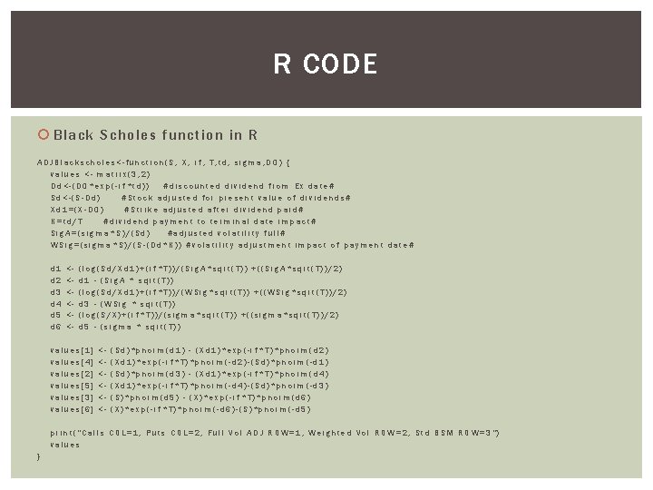
R CODE Black Scholes function in R ADJBlackscholes<-function(S, X, rf, T, td, sigma, D 0) { values <- matrix(3, 2) Dd<-(D 0*exp(-rf*td)) #discounted dividend from Ex date# Sd<-(S-Dd) #Stock adjusted for present value of dividends# Xd 1=(X-D 0) #Strike adjusted after dividend paid# K=td/T #dividend payment to terminal date impact# Sig. A=(sigma*S)/(Sd) #adjusted volatility full# WSig=(sigma*S)/(S-(Dd*K)) #volatility adjustment impact of payment date# d 1 d 2 d 3 d 4 d 5 d 6 <<<<<<- (log(Sd/Xd 1)+(rf*T))/(Sig. A*sqrt(T)) +((Sig. A*sqrt(T))/2) d 1 - (Sig. A * sqrt(T)) (log(Sd/Xd 1)+(rf*T))/(WSig*sqrt(T)) +((WSig*sqrt(T))/2) d 3 - (WSig * sqrt(T)) (log(S/X)+(rf*T))/(sigma*sqrt(T)) +((sigma*sqrt(T))/2) d 5 - (sigma * sqrt(T)) values[1] values[4] values[2] values[5] values[3] values[6] <<<<<<- (Sd)*pnorm(d 1) - (Xd 1)*exp(-rf*T)*pnorm(d 2) (Xd 1)*exp(-rf*T)*pnorm(-d 2)-(Sd)*pnorm(-d 1) (Sd)*pnorm(d 3) - (Xd 1)*exp(-rf*T)*pnorm(d 4) (Xd 1)*exp(-rf*T)*pnorm(-d 4)-(Sd)*pnorm(-d 3) (S)*pnorm(d 5) - (X)*exp(-rf*T)*pnorm(d 6) (X)*exp(-rf*T)*pnorm(-d 6)-(S)*pnorm(-d 5) print("Calls COL=1, Puts COL=2, Full Vol ADJ ROW=1, Weighted Vol ROW=2, Std BSM ROW=3") values }

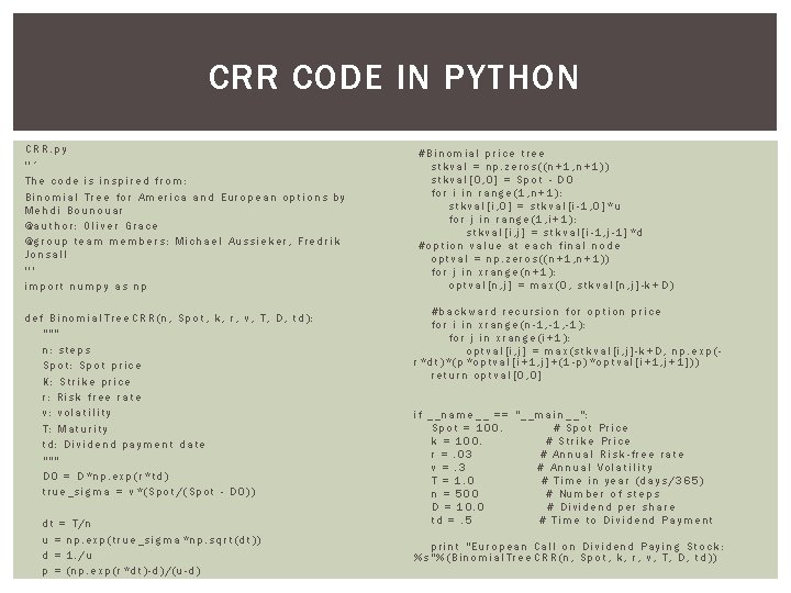
CRR CODE IN PYTHON CRR. py ''‘ The code is inspired from: Binomial Tree for America and European options by Mehdi Bounouar @author: Oliver Grace @group team members: Michael Aussieker, Fredrik Jonsall ''' import numpy as np def Binomial. Tree. CRR(n, Spot, k, r, v, T, D, td): """ n: steps Spot: Spot price K: Strike price r: Risk free rate v: volatility T: Maturity td: Dividend payment date """ D 0 = D*np. exp(r*td) true_sigma = v*(Spot/(Spot - D 0)) dt = T/n u = np. exp(true_sigma*np. sqrt(dt)) d = 1. /u p = (np. exp(r*dt)-d)/(u-d) #Binomial price tree stkval = np. zeros((n+1, n+1)) stkval[0, 0] = Spot - D 0 for i in range(1, n+1): stkval[i, 0] = stkval[i-1, 0]*u for j in range(1, i+1): stkval[i, j] = stkval[i-1, j-1]*d #option value at each final node optval = np. zeros((n+1, n+1)) for j in xrange(n+1): optval[n, j] = max(0, stkval[n, j]-k+D) #backward recursion for option price for i in xrange(n-1, -1): for j in xrange(i+1): optval[i, j] = max(stkval[i, j]-k+D, np. exp(r*dt)*(p*optval[i+1, j]+(1 -p)*optval[i+1, j+1])) return optval[0, 0] if __name__ == "__main__": Spot = 100. # Spot Price k = 100. # Strike Price r =. 03 # Annual Risk-free rate v =. 3 # Annual Volatility T = 1. 0 # Time in year (days/365) n = 500 # Number of steps D = 10. 0 # Dividend per share td =. 5 # Time to Dividend Payment print "European Call on Dividend Paying Stock: %s"%(Binomial. Tree. CRR(n, Spot, k, r, v, T, D, td))