Dr Kafu Wong ECON 1003 Analysis of Economic

Dr. Ka-fu Wong ECON 1003 Analysis of Economic Data Ka-fu Wong © 2003 Chap 11 - 1

Chapter Eleven Linear Regression and Correlation GOALS 1. 2. 3. 4. 5. 6. 7. l Draw a scatter diagram. Understand interpret the terms dependent variable and independent variable. Calculate and interpret the coefficient of correlation, the coefficient of determination, and the standard error of estimate. Conduct a test of hypothesis to determine if the population coefficient of correlation is different from zero. Calculate the least squares regression line and interpret the slope and intercept values. Construct and interpret a confidence interval and prediction interval for the dependent variable. Set up and interpret an ANOVA table. Ka-fu Wong © 2003 Chap 11 - 2

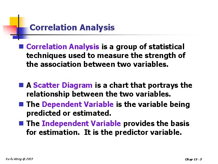
Correlation Analysis n Correlation Analysis is a group of statistical techniques used to measure the strength of the association between two variables. n A Scatter Diagram is a chart that portrays the relationship between the two variables. n The Dependent Variable is the variable being predicted or estimated. n The Independent Variable provides the basis for estimation. It is the predictor variable. Ka-fu Wong © 2003 Chap 11 - 3

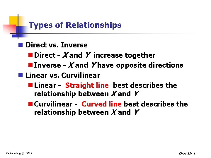
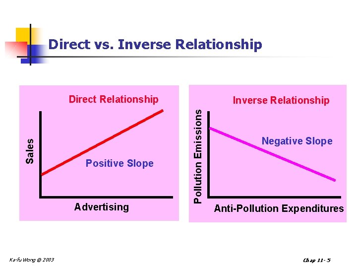
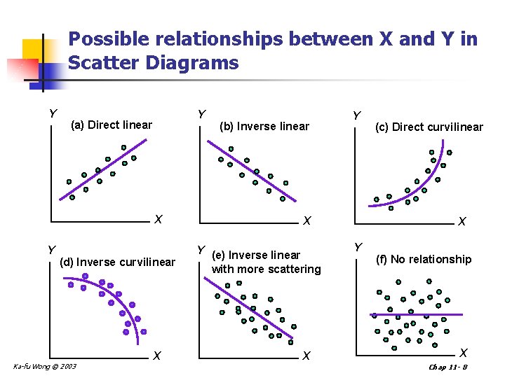
Types of Relationships n Direct vs. Inverse n Direct - X and Y increase together n Inverse - X and Y have opposite directions n Linear vs. Curvilinear n Linear - Straight line best describes the relationship between X and Y n Curvilinear - Curved line best describes the relationship between X and Y Ka-fu Wong © 2003 Chap 11 - 4

Direct vs. Inverse Relationship Positive Slope Advertising Ka-fu Wong © 2003 Inverse Relationship Pollution Emissions Sales Direct Relationship Negative Slope Anti-Pollution Expenditures Chap 11 - 5

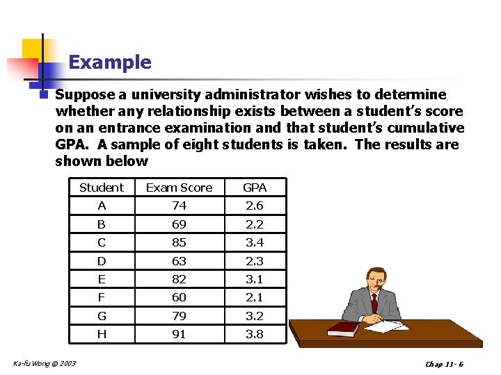
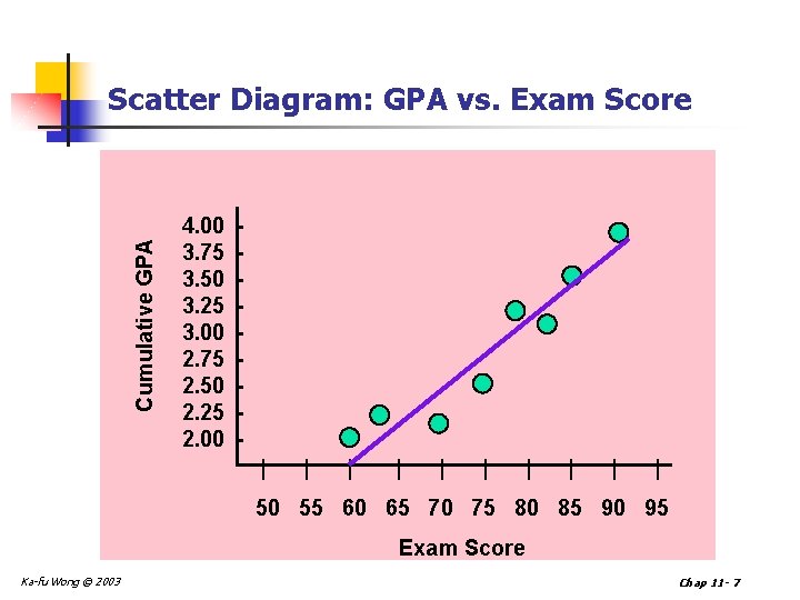
Example n Suppose a university administrator wishes to determine whether any relationship exists between a student’s score on an entrance examination and that student’s cumulative GPA. A sample of eight students is taken. The results are shown below Ka-fu Wong © 2003 Student Exam Score GPA A 74 2. 6 B 69 2. 2 C 85 3. 4 D 63 2. 3 E 82 3. 1 F 60 2. 1 G 79 3. 2 H 91 3. 8 Chap 11 - 6

Cumulative GPA Scatter Diagram: GPA vs. Exam Score 4. 00 3. 75 3. 50 3. 25 3. 00 2. 75 2. 50 2. 25 2. 00 | | | | | 50 55 60 65 70 75 80 85 90 95 Exam Score Ka-fu Wong © 2003 Chap 11 - 7

Possible relationships between X and Y in Scatter Diagrams Y Y (a) Direct linear X Y (d) Inverse curvilinear Ka-fu Wong © 2003 X (b) Inverse linear Y X Y (e) Inverse linear with more scattering X (c) Direct curvilinear X Y (f) No relationship X Chap 11 - 8

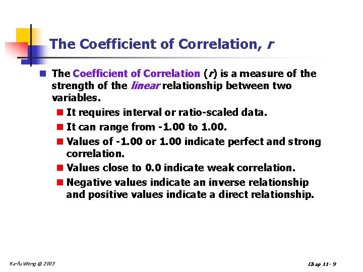
The Coefficient of Correlation, r n The Coefficient of Correlation (r) is a measure of the strength of the linear relationship between two variables. n It requires interval or ratio-scaled data. n It can range from -1. 00 to 1. 00. n Values of -1. 00 or 1. 00 indicate perfect and strong correlation. n Values close to 0. 0 indicate weak correlation. n Negative values indicate an inverse relationship and positive values indicate a direct relationship. Ka-fu Wong © 2003 Chap 11 - 9

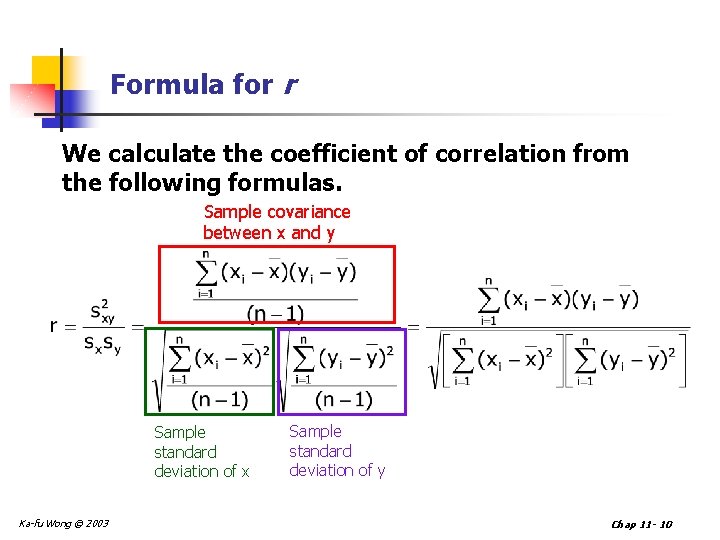
Formula for r We calculate the coefficient of correlation from the following formulas. Sample covariance between x and y Sample standard deviation of x Ka-fu Wong © 2003 Sample standard deviation of y Chap 11 - 10

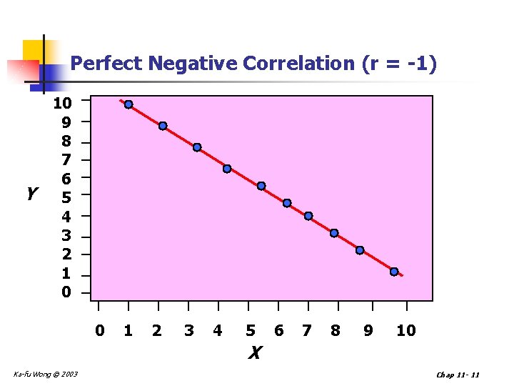
Perfect Negative Correlation (r = -1) Y 10 9 8 7 6 5 4 3 2 1 0 0 1 2 3 4 5 6 7 8 9 10 X Ka-fu Wong © 2003 Chap 11 - 11

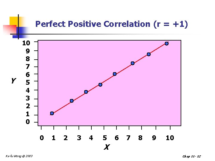
Perfect Positive Correlation (r = +1) Y 10 9 8 7 6 5 4 3 2 1 0 0 1 2 3 4 5 6 7 8 9 10 X Ka-fu Wong © 2003 Chap 11 - 12

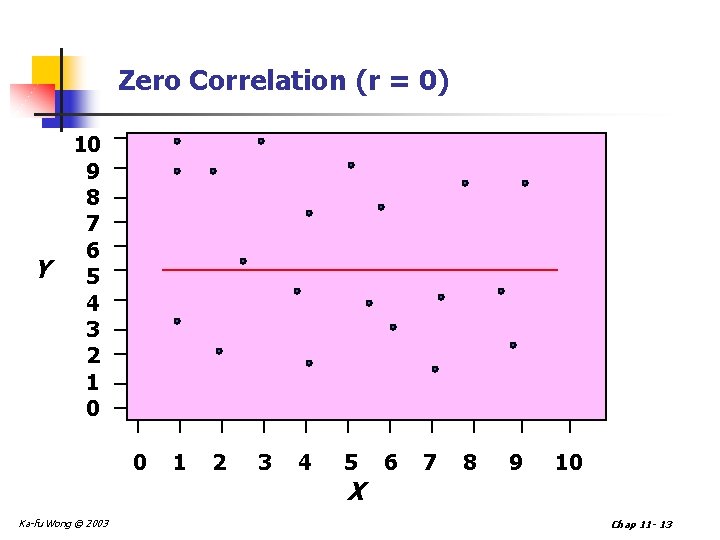
Zero Correlation (r = 0) Y 10 9 8 7 6 5 4 3 2 1 0 0 1 2 3 4 5 6 7 8 9 10 X Ka-fu Wong © 2003 Chap 11 - 13

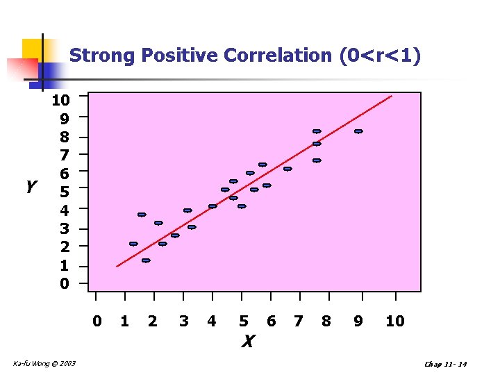
Strong Positive Correlation (0<r<1) Y 10 9 8 7 6 5 4 3 2 1 0 0 1 2 3 4 5 6 7 8 9 10 X Ka-fu Wong © 2003 Chap 11 - 14

Coefficient of Determination n The coefficient of determination (r 2) is the proportion of the total variation in the dependent variable (Y) that is explained or accounted for by the variation in the independent variable (X). n It is the square of the coefficient of correlation. n It ranges from 0 to 1. n It does not give any information on the direction of the relationship between the variables. n Special cases: n No correlation: r=0, r 2=0. n Perfect negative correlation: r=-1, r 2=1. n Perfect positive correlation: r=+1, r 2=1. Ka-fu Wong © 2003 Chap 11 - 15

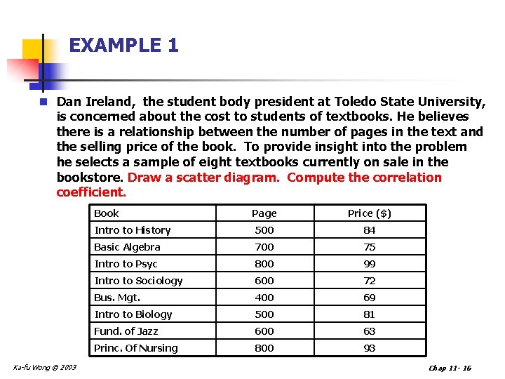
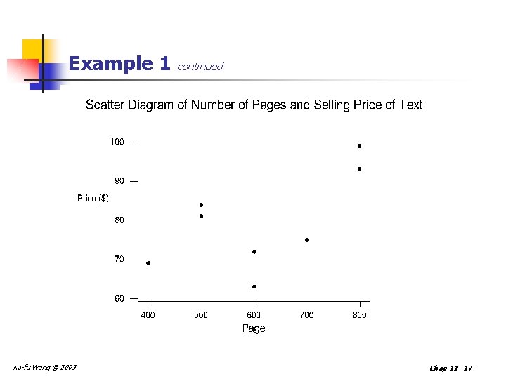
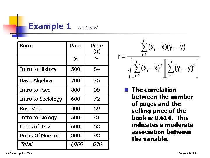
EXAMPLE 1 n Dan Ireland, the student body president at Toledo State University, is concerned about the cost to students of textbooks. He believes there is a relationship between the number of pages in the text and the selling price of the book. To provide insight into the problem he selects a sample of eight textbooks currently on sale in the bookstore. Draw a scatter diagram. Compute the correlation coefficient. Ka-fu Wong © 2003 Book Page Price ($) Intro to History 500 84 Basic Algebra 700 75 Intro to Psyc 800 99 Intro to Sociology 600 72 Bus. Mgt. 400 69 Intro to Biology 500 81 Fund. of Jazz 600 63 Princ. Of Nursing 800 93 Chap 11 - 16

Example 1 continued Ka-fu Wong © 2003 Chap 11 - 17

Example 1 Book continued Page Price ($) X Y Intro to History 500 84 Basic Algebra 700 75 Intro to Psyc 800 99 Intro to Sociology 600 72 Bus. Mgt. 400 69 Intro to Biology 500 81 Fund. of Jazz 600 63 Princ. Of Nursing 800 93 4, 900 636 Total Ka-fu Wong © 2003 n The correlation between the number of pages and the selling price of the book is 0. 614. This indicates a moderate association between the variable. Chap 11 - 18

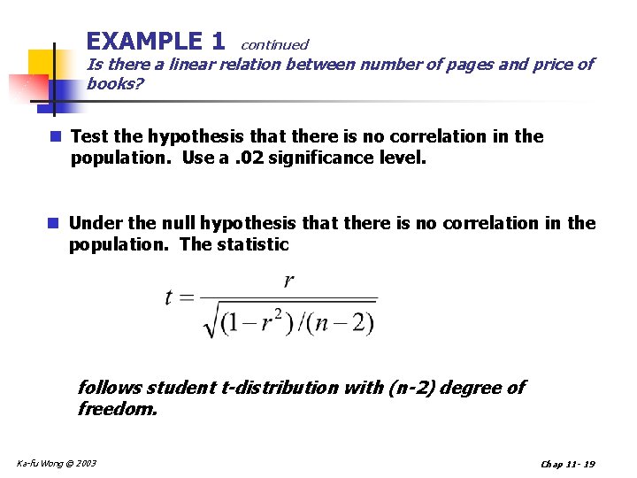
EXAMPLE 1 continued Is there a linear relation between number of pages and price of books? n Test the hypothesis that there is no correlation in the population. Use a. 02 significance level. n Under the null hypothesis that there is no correlation in the population. The statistic follows student t-distribution with (n-2) degree of freedom. Ka-fu Wong © 2003 Chap 11 - 19

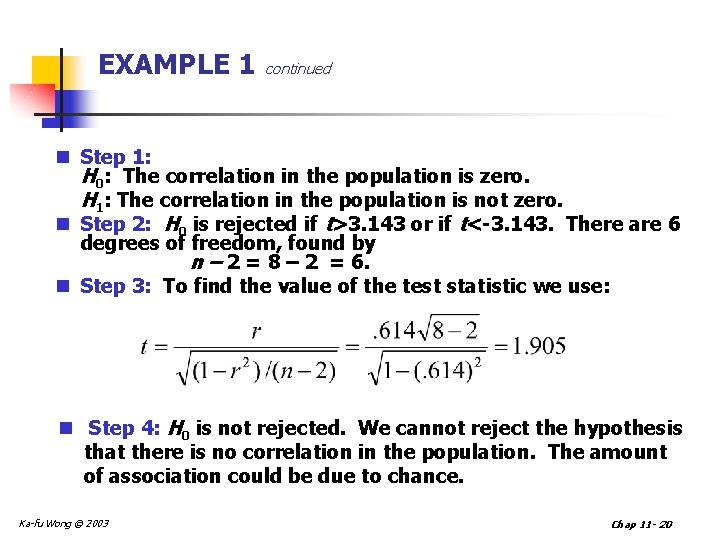
EXAMPLE 1 continued n Step 1: H 0: The correlation in the population is zero. H 1: The correlation in the population is not zero. n Step 2: H 0 is rejected if t>3. 143 or if t<-3. 143. There are 6 degrees of freedom, found by n – 2 = 8 – 2 = 6. n Step 3: To find the value of the test statistic we use: n Step 4: H 0 is not rejected. We cannot reject the hypothesis that there is no correlation in the population. The amount of association could be due to chance. Ka-fu Wong © 2003 Chap 11 - 20

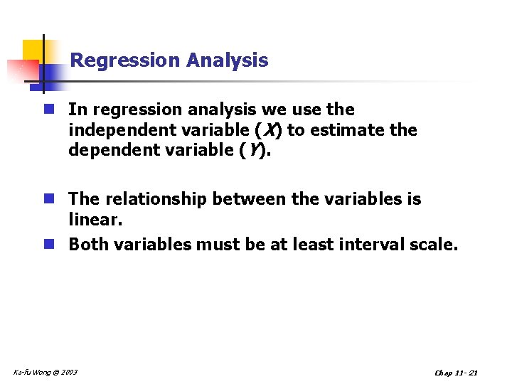
Regression Analysis n In regression analysis we use the independent variable (X) to estimate the dependent variable (Y). n The relationship between the variables is linear. n Both variables must be at least interval scale. Ka-fu Wong © 2003 Chap 11 - 21

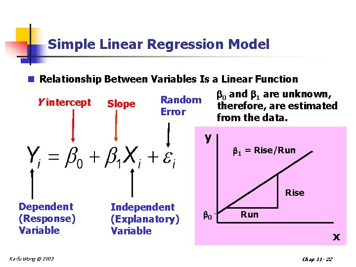
Simple Linear Regression Model n Relationship Between Variables Is a Linear Function 0 and 1 are unknown, Random Y intercept Slope therefore, are estimated Error from the data. y 1 = Rise/Run Rise Dependent (Response) Variable Ka-fu Wong © 2003 Independent (Explanatory) Variable 0 Run x Chap 11 - 22

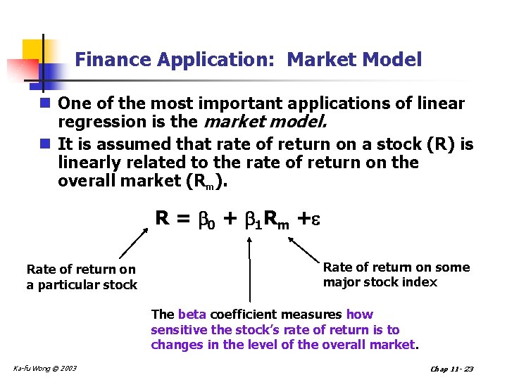
Finance Application: Market Model n One of the most important applications of linear regression is the market model. n It is assumed that rate of return on a stock (R) is linearly related to the rate of return on the overall market (Rm). R = 0 + 1 Rm + Rate of return on a particular stock Rate of return on some major stock index The beta coefficient measures how sensitive the stock’s rate of return is to changes in the level of the overall market. Ka-fu Wong © 2003 Chap 11 - 23

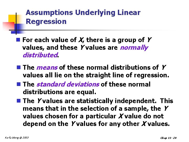
Assumptions Underlying Linear Regression n For each value of X, there is a group of Y values, and these Y values are normally distributed. n The means of these normal distributions of Y values all lie on the straight line of regression. n The standard deviations of these normal distributions are equal. n The Y values are statistically independent. This means that in the selection of a sample, the Y values chosen for a particular X value do not depend on the Y values for any other X values. Ka-fu Wong © 2003 Chap 11 - 24

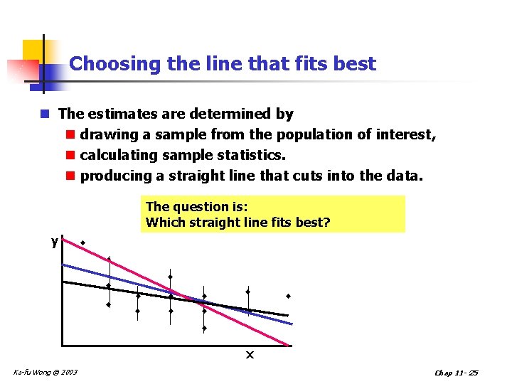
Choosing the line that fits best n The estimates are determined by n drawing a sample from the population of interest, n calculating sample statistics. n producing a straight line that cuts into the data. The question is: Which straight line fits best? y w w w w x Ka-fu Wong © 2003 Chap 11 - 25

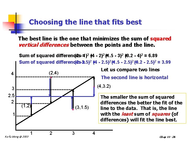
Choosing the line that fits best The best line is the one that minimizes the sum of squared vertical differences between the points and the line. Sum of squared differences (2 - =1)2 + (4 - 2)2 (+1. 5 - 3)2 + (3. 2 - 4)2 = 6. 89 Sum of squared differences (2 -2. 5) = 2+ (4 - 2. 5)2 (+1. 5 - 2. 5)2 (3. 2 + - 2. 5)2 = 3. 99 3 2. 5 2 Let us compare two lines (2, 4) w 4 The second line is horizontal w (4, 3. 2) (1, 2)w w (3, 1. 5) 1 Ka-fu Wong © 2003 1 The smaller the sum of squared differences the better the fit of the line to the data. That is, the line with the least sum of squares (of differences) will fit the line best. 2 3 4 Chap 11 - 26

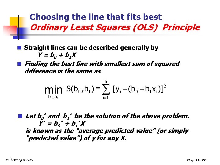
Choosing the line that fits best Ordinary Least Squares (OLS) Principle n Straight lines can be described generally by Y = b 0 + b 1 X n Finding the best line with smallest sum of squared difference is the same as n Let b 0* and b 1* be the solution of the above problem. Y* = b 0* + b 1*X is known as the “average predicted value” (or simply “predicted value”) of y for any X. Ka-fu Wong © 2003 Chap 11 - 27

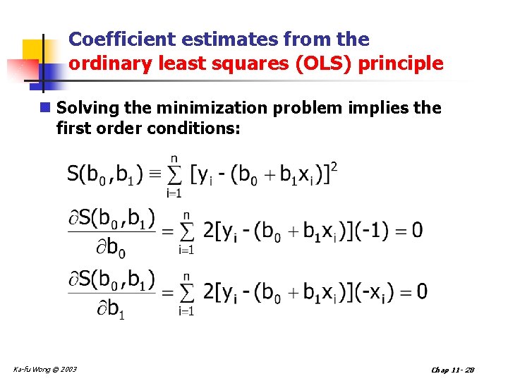
Coefficient estimates from the ordinary least squares (OLS) principle n Solving the minimization problem implies the first order conditions: Ka-fu Wong © 2003 Chap 11 - 28

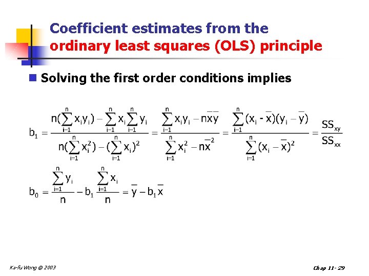
Coefficient estimates from the ordinary least squares (OLS) principle n Solving the first order conditions implies Ka-fu Wong © 2003 Chap 11 - 29

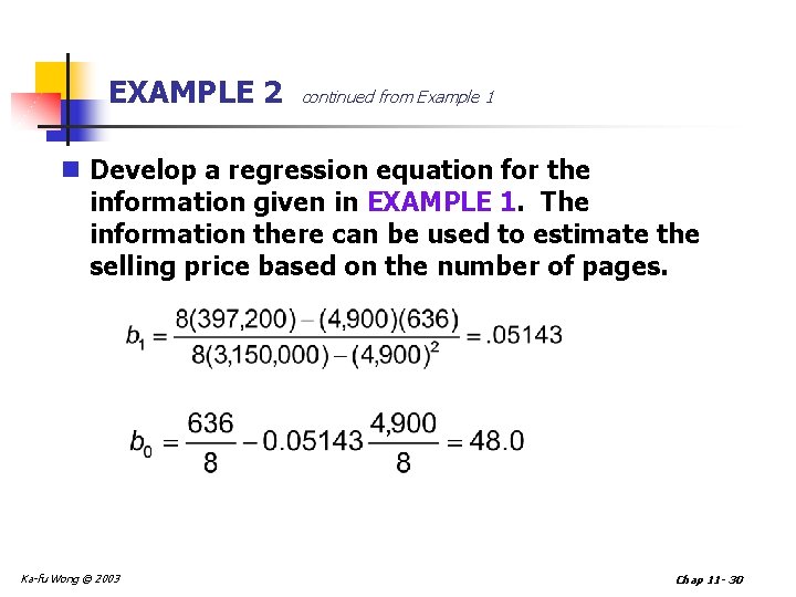
EXAMPLE 2 continued from Example 1 n Develop a regression equation for the information given in EXAMPLE 1. The information there can be used to estimate the selling price based on the number of pages. Ka-fu Wong © 2003 Chap 11 - 30

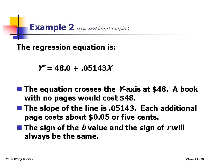
Example 2 continued from Example 1 The regression equation is: Y* = 48. 0 +. 05143 X n The equation crosses the Y-axis at $48. A book with no pages would cost $48. n The slope of the line is. 05143. Each additional page costs about $0. 05 or five cents. n The sign of the b value and the sign of r will always be the same. Ka-fu Wong © 2003 Chap 11 - 31

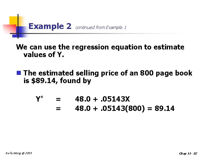
Example 2 continued from Example 1 We can use the regression equation to estimate values of Y. n The estimated selling price of an 800 page book is $89. 14, found by Y* Ka-fu Wong © 2003 = = 48. 0 +. 05143 X 48. 0 +. 05143(800) = 89. 14 Chap 11 - 32

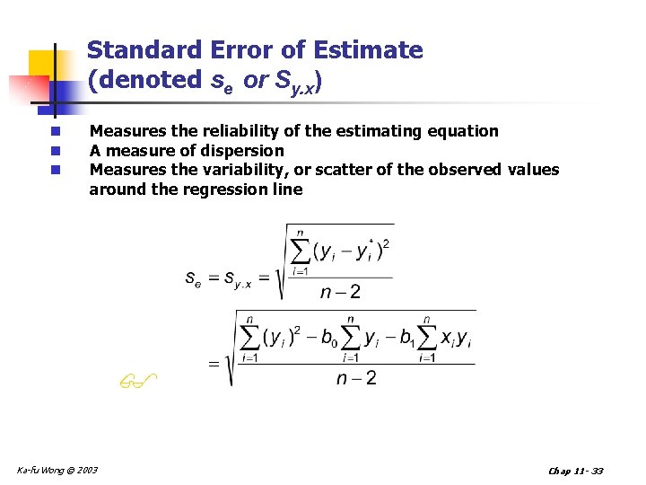
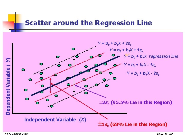
Standard Error of Estimate (denoted se or Sy. x) n n n Measures the reliability of the estimating equation A measure of dispersion Measures the variability, or scatter of the observed values around the regression line Ka-fu Wong © 2003 Chap 11 - 33

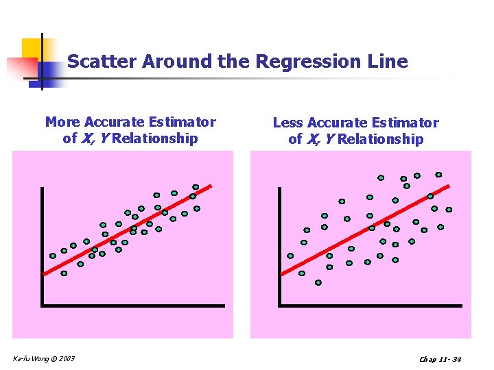
Scatter Around the Regression Line More Accurate Estimator of X, Y Relationship Ka-fu Wong © 2003 Less Accurate Estimator of X, Y Relationship Chap 11 - 34

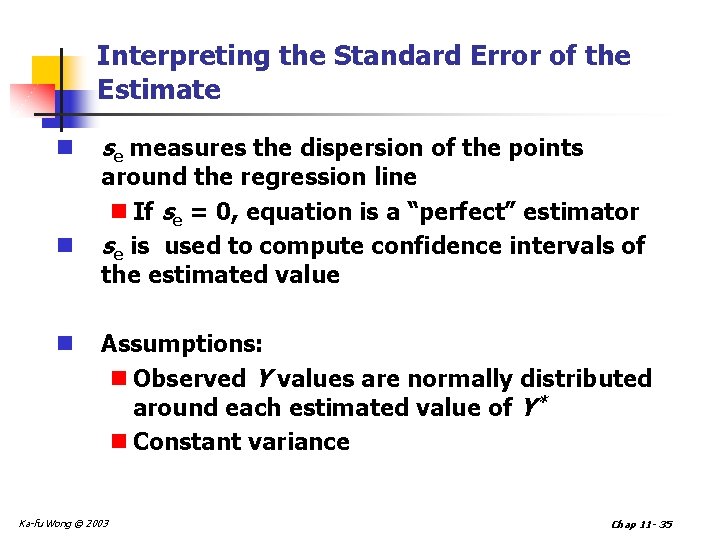
Interpreting the Standard Error of the Estimate n n n se measures the dispersion of the points around the regression line n If se = 0, equation is a “perfect” estimator se is used to compute confidence intervals of the estimated value Assumptions: n Observed Y values are normally distributed around each estimated value of Y* n Constant variance Ka-fu Wong © 2003 Chap 11 - 35

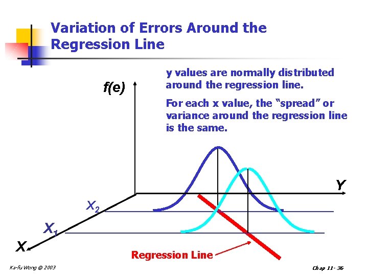
Variation of Errors Around the Regression Line f(e) y values are normally distributed around the regression line. For each x value, the “spread” or variance around the regression line is the same. Y X 2 X X 1 Ka-fu Wong © 2003 Regression Line Chap 11 - 36

Scatter around the Regression Line Y = b 0 + b 1 X + 2 se Dependent Variable ( Y) Y = b 0 + b 1 X + 1 se Y = b 0 + b 1 X regression line Y = b 0 + b 1 X - 1 se Y = b 0 + b 1 X - 2 se (95. 5% Lie in this Region) Independent Variable (X) Ka-fu Wong © 2003 1 se (68% Lie in this Region) Chap 11 - 37

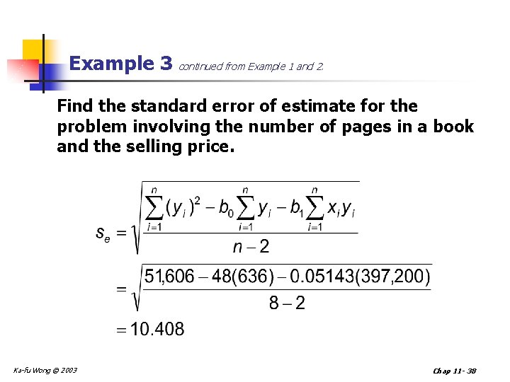
Example 3 continued from Example 1 and 2. Find the standard error of estimate for the problem involving the number of pages in a book and the selling price. Ka-fu Wong © 2003 Chap 11 - 38

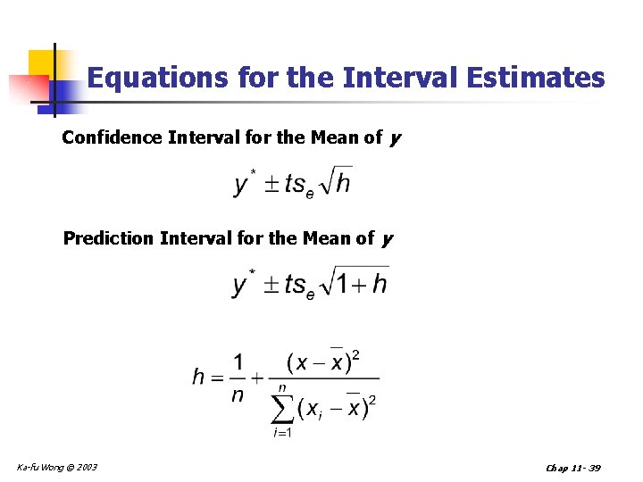
Equations for the Interval Estimates Confidence Interval for the Mean of y Prediction Interval for the Mean of y Ka-fu Wong © 2003 Chap 11 - 39

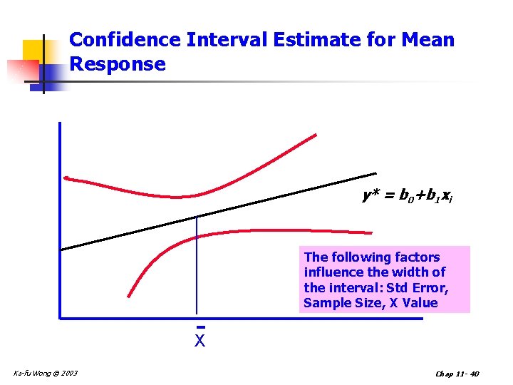
Confidence Interval Estimate for Mean Response y* = b 0+b 1 xi The following factors influence the width of the interval: Std Error, Sample Size, X Value X Ka-fu Wong © 2003 Chap 11 - 40

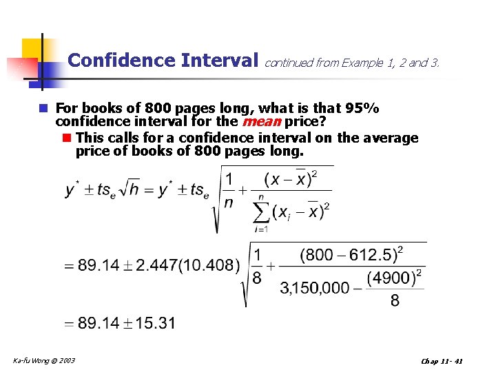
Confidence Interval continued from Example 1, 2 and 3. n For books of 800 pages long, what is that 95% confidence interval for the mean price? n This calls for a confidence interval on the average price of books of 800 pages long. Ka-fu Wong © 2003 Chap 11 - 41

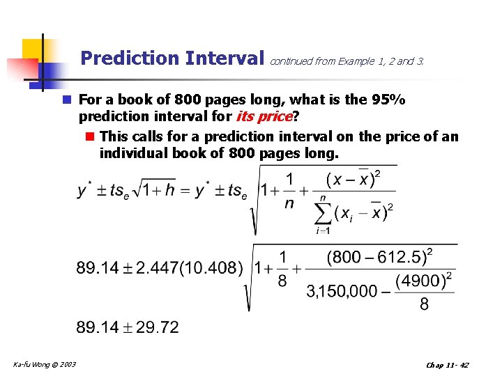
Prediction Interval continued from Example 1, 2 and 3. n For a book of 800 pages long, what is the 95% prediction interval for its price? n This calls for a prediction interval on the price of an individual book of 800 pages long. Ka-fu Wong © 2003 Chap 11 - 42

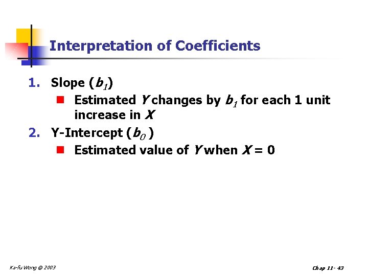
Interpretation of Coefficients 1. Slope (b 1) n Estimated Y changes by b 1 for each 1 unit increase in X 2. Y-Intercept (b 0 ) n Estimated value of Y when X = 0 Ka-fu Wong © 2003 Chap 11 - 43

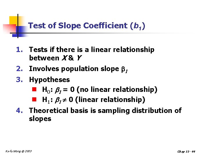
Test of Slope Coefficient (b 1) 1. Tests if there is a linear relationship between X & Y 2. Involves population slope 1 3. Hypotheses n H 0: b 1 = 0 (no linear relationship) n H 1: b 1 0 (linear relationship) 4. Theoretical basis is sampling distribution of slopes Ka-fu Wong © 2003 Chap 11 - 44

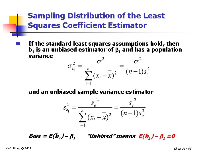
Sampling Distribution of the Least Squares Coefficient Estimator n If the standard least squares assumptions hold, then b 1 is an unbiased estimator of 1 and has a population variance and an unbiased sample variance estimator Bias = E(b 1) - b 1 Ka-fu Wong © 2003 “Unbiasd” means E(b 1) - b 1 =0 Chap 11 - 45

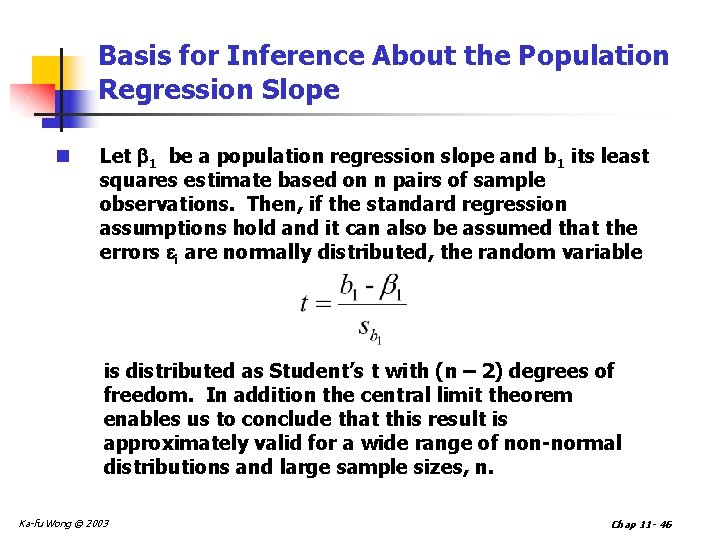
Basis for Inference About the Population Regression Slope n Let 1 be a population regression slope and b 1 its least squares estimate based on n pairs of sample observations. Then, if the standard regression assumptions hold and it can also be assumed that the errors i are normally distributed, the random variable is distributed as Student’s t with (n – 2) degrees of freedom. In addition the central limit theorem enables us to conclude that this result is approximately valid for a wide range of non-normal distributions and large sample sizes, n. Ka-fu Wong © 2003 Chap 11 - 46

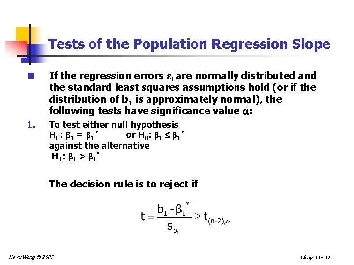
Tests of the Population Regression Slope n If the regression errors i are normally distributed and the standard least squares assumptions hold (or if the distribution of b 1 is approximately normal), the following tests have significance value : 1. To test either null hypothesis H 0 : 1 = 1 * or H 0: 1 1* against the alternative H 1 : 1 > 1 * The decision rule is to reject if Ka-fu Wong © 2003 Chap 11 - 47

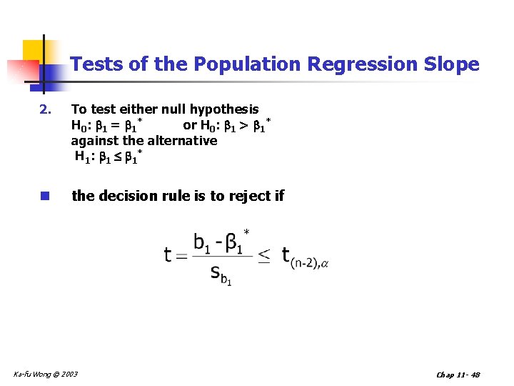
Tests of the Population Regression Slope 2. To test either null hypothesis H 0 : 1 = 1 * or H 0: 1 > 1* against the alternative H 1 : 1 1 * n the decision rule is to reject if Ka-fu Wong © 2003 Chap 11 - 48

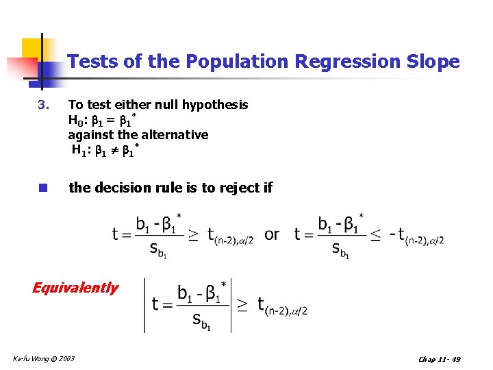
Tests of the Population Regression Slope 3. To test either null hypothesis H 0 : 1 = 1 * against the alternative H 1 : 1 1 * n the decision rule is to reject if Equivalently Ka-fu Wong © 2003 Chap 11 - 49

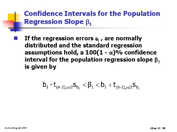
Confidence Intervals for the Population Regression Slope 1 n If the regression errors i , are normally distributed and the standard regression assumptions hold, a 100(1 - )% confidence interval for the population regression slope 1 is given by Ka-fu Wong © 2003 Chap 11 - 50

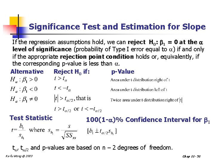
Significance Test and Estimation for Slope If the regression assumptions hold, we can reject H 0: 1 = 0 at the level of significance (probability of Type I error equal to ) if and only if the appropriate rejection point condition holds or, equivalently, if the corresponding p-value is less than . p-Value Alternative Reject H 0 if: Test Statistic 100(1 - )% Confidence Interval for 1 t , t /2 and p-values are based on n – 2 degrees of freedom. Ka-fu Wong © 2003 Chap 11 - 51

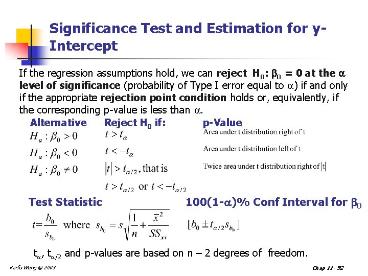
Significance Test and Estimation for y. Intercept If the regression assumptions hold, we can reject H 0: 0 = 0 at the level of significance (probability of Type I error equal to ) if and only if the appropriate rejection point condition holds or, equivalently, if the corresponding p-value is less than . p-Value Alternative Reject H 0 if: Test Statistic 100(1 - )% Conf Interval for 0 t , t /2 and p-values are based on n – 2 degrees of freedom. Ka-fu Wong © 2003 Chap 11 - 52

Some cautions about the interpretation of significance tests n Rejecting H 0: b 1 = 0 and concluding that the relationship between x and y is significant does not enable us to conclude that a cause-and-effect relationship is present between x and y. n Causation requires: n Association n Accurate time sequence n Other explanation for correlation Correlation Causation Ka-fu Wong © 2003 Chap 11 - 53

Some cautions about the interpretation of significance tests n Just because we are able to reject H 0: b 1 = 0 and demonstrate statistical significance does not enable us to conclude that there is a linear relationship between x and y. n Linear relationship is a very small subset of possible relationship among variables. n A test of linear versus nonlinear relationship requires another batch of analysis. Ka-fu Wong © 2003 Chap 11 - 54

Evaluating the Model n Variation Measures n Coeff. Of Determination n Standard Error of Estimate n Test Coefficients for Significance yi* = b 0 +b 1 xi Ka-fu Wong © 2003 Chap 11 - 55

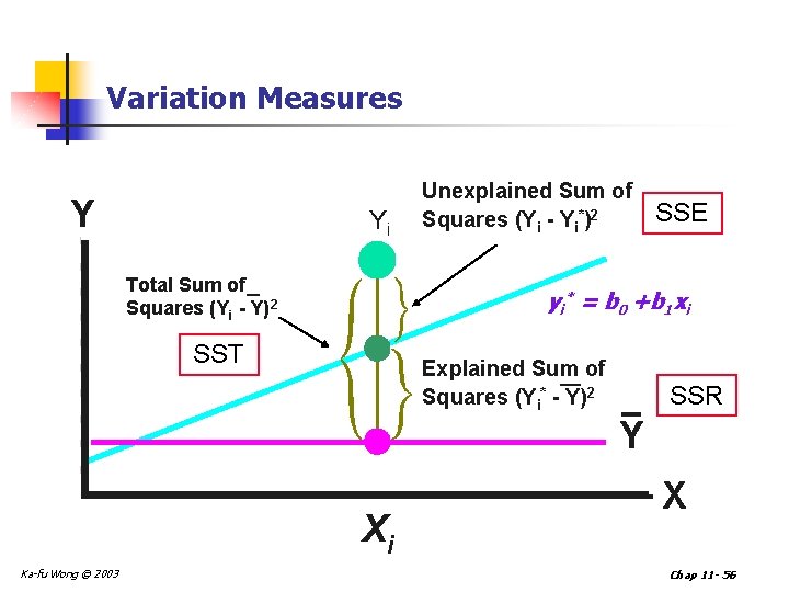
Variation Measures Y Yi Total Sum of Squares (Yi - Y)2 Unexplained Sum of Squares (Yi - Yi*)2 SSE yi* = b 0 +b 1 xi SST Explained Sum of Squares (Yi* - Y)2 SSR Y Xi Ka-fu Wong © 2003 X Chap 11 - 56

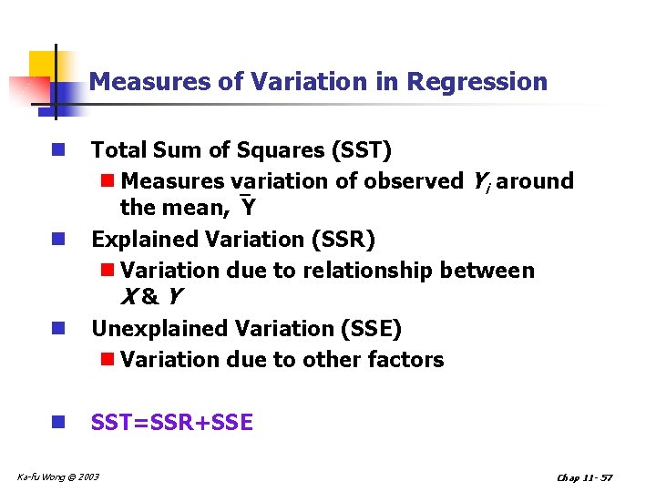
Measures of Variation in Regression n n Total Sum of Squares (SST) n Measures variation of observed Yi around the mean, Y Explained Variation (SSR) n Variation due to relationship between X&Y Unexplained Variation (SSE) n Variation due to other factors SST=SSR+SSE Ka-fu Wong © 2003 Chap 11 - 57

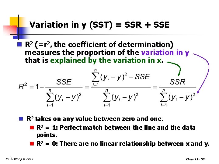
Variation in y (SST) = SSR + SSE n R 2 (=r 2, the coefficient of determination) measures the proportion of the variation in y that is explained by the variation in x. n R 2 takes on any value between zero and one. n R 2 = 1: Perfect match between the line and the data points. n R 2 = 0: There are no linear relationship between x and y. Ka-fu Wong © 2003 Chap 11 - 58

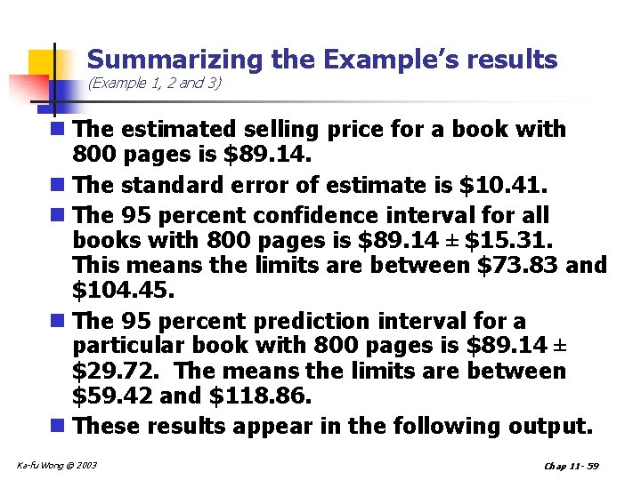
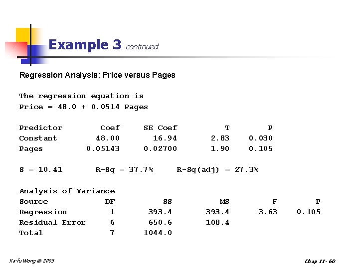
Summarizing the Example’s results (Example 1, 2 and 3) n The estimated selling price for a book with 800 pages is $89. 14. n The standard error of estimate is $10. 41. n The 95 percent confidence interval for all books with 800 pages is $89. 14 ± $15. 31. This means the limits are between $73. 83 and $104. 45. n The 95 percent prediction interval for a particular book with 800 pages is $89. 14 ± $29. 72. The means the limits are between $59. 42 and $118. 86. n These results appear in the following output. Ka-fu Wong © 2003 Chap 11 - 59

Example 3 continued Regression Analysis: Price versus Pages The regression equation is Price = 48. 0 + 0. 0514 Pages Predictor Constant Pages S = 10. 41 Coef 48. 00 0. 05143 R-Sq = 37. 7% Analysis of Variance Source DF Regression 1 Residual Error 6 Total 7 Ka-fu Wong © 2003 SE Coef 16. 94 0. 02700 SS 393. 4 650. 6 1044. 0 T 2. 83 1. 90 P 0. 030 0. 105 R-Sq(adj) = 27. 3% MS 393. 4 108. 4 F 3. 63 P 0. 105 Chap 11 - 60

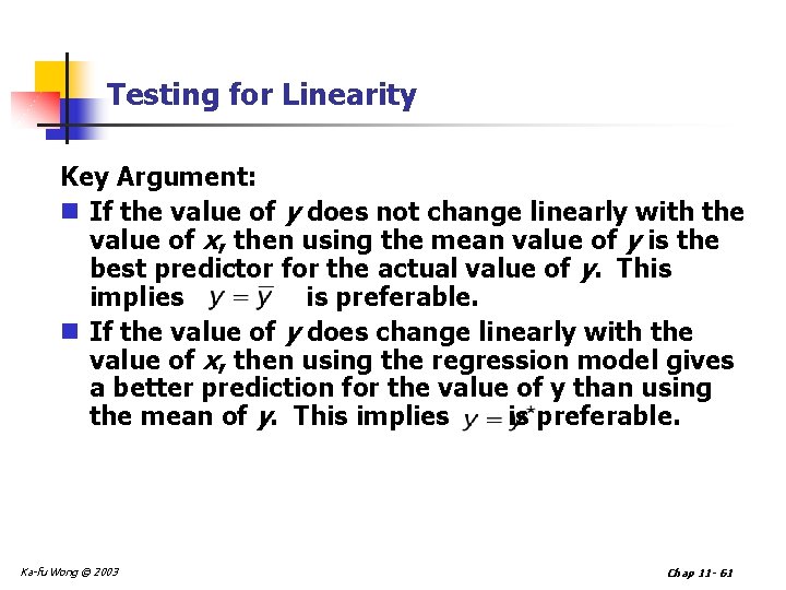
Testing for Linearity Key Argument: n If the value of y does not change linearly with the value of x, then using the mean value of y is the best predictor for the actual value of y. This implies is preferable. n If the value of y does change linearly with the value of x, then using the regression model gives a better prediction for the value of y than using the mean of y. This implies is preferable. Ka-fu Wong © 2003 Chap 11 - 61

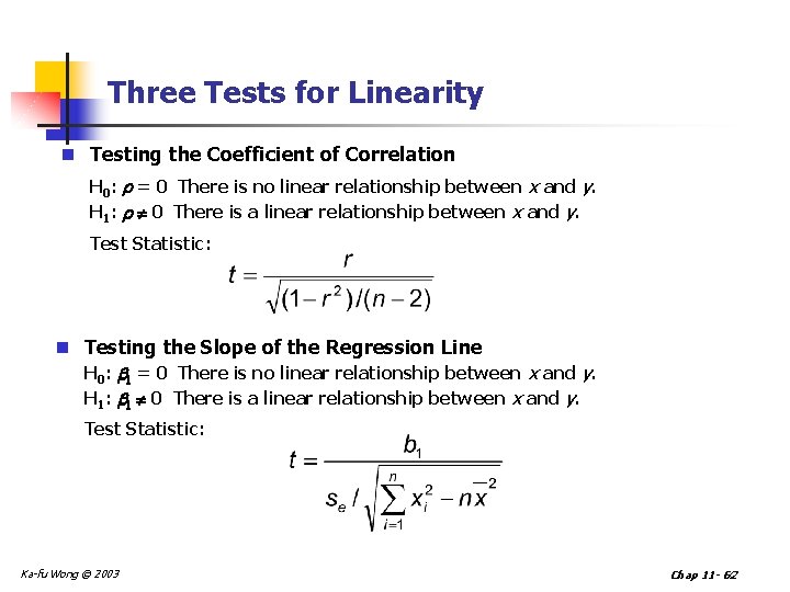
Three Tests for Linearity n Testing the Coefficient of Correlation H 0: r = 0 There is no linear relationship between x and y. H 1: r 0 There is a linear relationship between x and y. Test Statistic: n Testing the Slope of the Regression Line H 0: b 1 = 0 There is no linear relationship between x and y. H 1: b 1 0 There is a linear relationship between x and y. Test Statistic: Ka-fu Wong © 2003 Chap 11 - 62

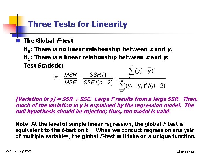
Three Tests for Linearity n The Global F-test H 0: There is no linear relationship between x and y. H 1: There is a linear relationship between x and y. Test Statistic: [Variation in y] = SSR + SSE. Large F results from a large SSR. Then, much of the variation in y is explained by the regression model. The null hypothesis should be rejected; thus, the model is valid. Note: At the level of simple linear regression, the global F-test is equivalent to the t-test on b 1. When we conduct regression analysis of multiple variables, the global F-test will take on a unique function. Ka-fu Wong © 2003 Chap 11 - 63

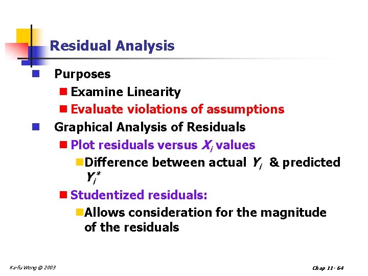
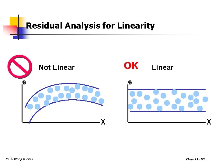
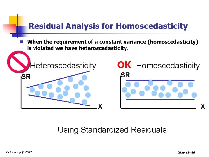
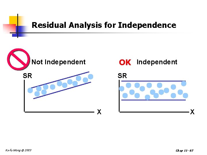
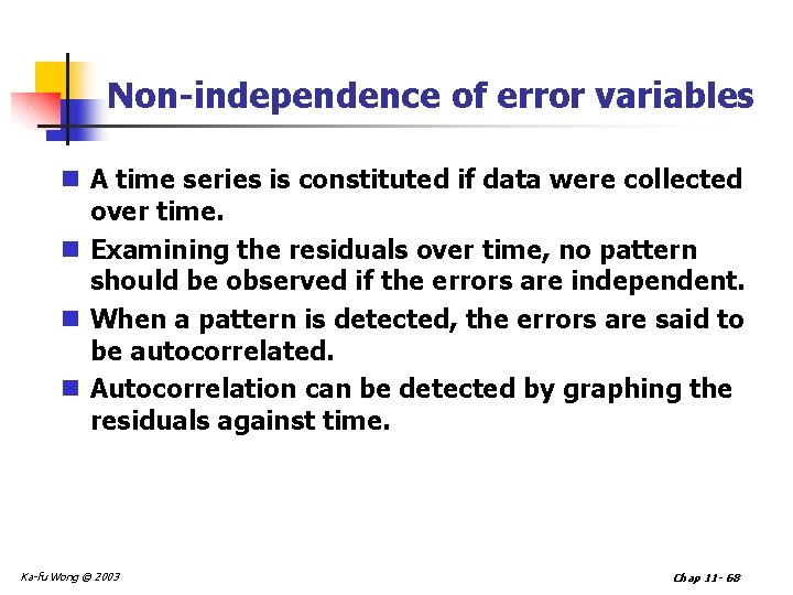
Residual Analysis n n Purposes n Examine Linearity n Evaluate violations of assumptions Graphical Analysis of Residuals n Plot residuals versus Xi values n. Difference between actual Yi & predicted Yi* n Studentized residuals: n. Allows consideration for the magnitude of the residuals Ka-fu Wong © 2003 Chap 11 - 64

Residual Analysis for Linearity OK Not Linear e X Ka-fu Wong © 2003 X Chap 11 - 65

Residual Analysis for Homoscedasticity n When the requirement of a constant variance (homoscedasticity) is violated we have heteroscedasticity. OK Homoscedasticity Heteroscedasticity SR SR X X Using Standardized Residuals Ka-fu Wong © 2003 Chap 11 - 66

Residual Analysis for Independence OK Independent Not Independent SR SR X Ka-fu Wong © 2003 X Chap 11 - 67

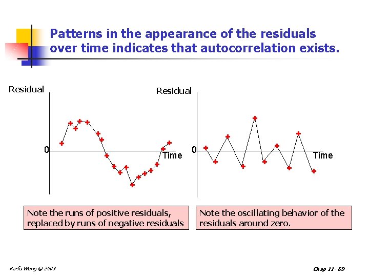
Non-independence of error variables n A time series is constituted if data were collected over time. n Examining the residuals over time, no pattern should be observed if the errors are independent. n When a pattern is detected, the errors are said to be autocorrelated. n Autocorrelation can be detected by graphing the residuals against time. Ka-fu Wong © 2003 Chap 11 - 68

Patterns in the appearance of the residuals over time indicates that autocorrelation exists. Residual + ++ + 0 + + ++ + 0 + Time Note the runs of positive residuals, replaced by runs of negative residuals Ka-fu Wong © 2003 + + + Time + + Note the oscillating behavior of the residuals around zero. Chap 11 - 69

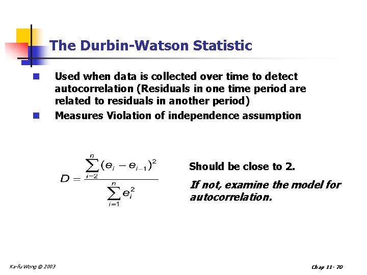
The Durbin-Watson Statistic n n Used when data is collected over time to detect autocorrelation (Residuals in one time period are related to residuals in another period) Measures Violation of independence assumption Should be close to 2. If not, examine the model for autocorrelation. Ka-fu Wong © 2003 Chap 11 - 70

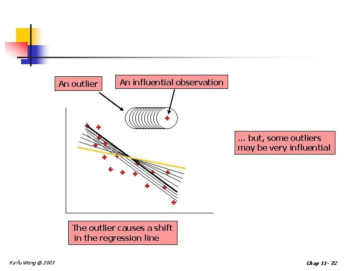
Outliers n An outlier is an observation that is unusually small or large. n Several possibilities need to be investigated when an outlier is observed: n There was an error in recording the value. n The point does not belong in the sample. n The observation is valid. n Identify outliers from the scatter diagram. n It is customary to suspect an observation is an outlier if its |standard residual| > 2 Ka-fu Wong © 2003 Chap 11 - 71

An outlier An influential observation + + + + ++++++ … but, some outliers may be very influential + + + + The outlier causes a shift in the regression line Ka-fu Wong © 2003 Chap 11 - 72

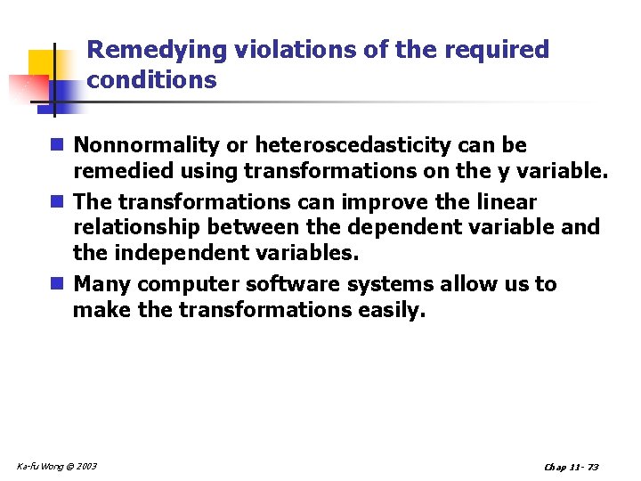
Remedying violations of the required conditions n Nonnormality or heteroscedasticity can be remedied using transformations on the y variable. n The transformations can improve the linear relationship between the dependent variable and the independent variables. n Many computer software systems allow us to make the transformations easily. Ka-fu Wong © 2003 Chap 11 - 73

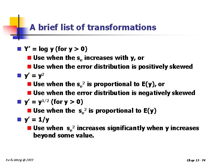
A brief list of transformations n Y’ = log y (for y > 0) n Use when the se increases with y, or n Use when the error distribution is positively skewed n y’ = y 2 n Use when the se 2 is proportional to E(y), or n Use when the error distribution is negatively skewed n y’ = y 1/2 (for y > 0) n Use when the se 2 is proportional to E(y) n y’ = 1/y n Use when se 2 increases significantly when y increases beyond some value. Ka-fu Wong © 2003 Chap 11 - 74

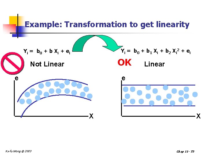
Example: Transformation to get linearity Yi = b 0 + b 1 X i + b 2 X i 2 + e i Yi = b 0 + b X i + e i OK Not Linear e X Ka-fu Wong © 2003 X Chap 11 - 75

Chapter Eleven Linear Regression and Correlation - END - Ka-fu Wong © 2003 Chap 11 - 76