Dr Kafu Wong ECON 1003 Analysis of Economic

Dr. Ka-fu Wong ECON 1003 Analysis of Economic Data Ka-fu Wong © 2003 Chap 7 - 1

Chapter Seven The Normal Probability Distribution GOALS 1. 2. 3. 4. 5. 6. l List the characteristics of the normal probability distribution. Define and calculate z values. Determine the probability an observation will lie between two points using the standard normal distribution. Determine the probability an observation will be above or below a given value using the standard normal distribution. Compare two or more observations that are on different probability distributions. Use the normal distribution to approximate the binomial probability distribution. Ka-fu Wong © 2003 Chap 7 - 2

Importance of Normal Distribution 1. Describes many random processes or continuous phenomena 2. Basis for Statistical Inference Ka-fu Wong © 2003 Chap 7 - 3

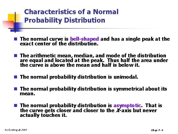
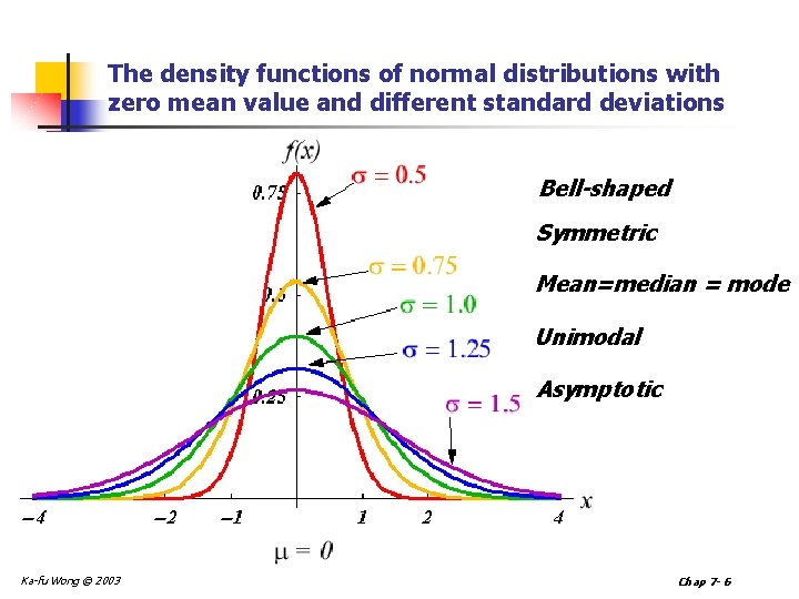
Characteristics of a Normal Probability Distribution n The normal curve is bell-shaped and has a single peak at the exact center of the distribution. n The arithmetic mean, median, and mode of the distribution are equal and located at the peak. Thus half the area under the curve is above the mean and half is below it. n The normal probability distribution is unimodal. n The normal probability distribution is symmetrical about its mean. n The normal probability distribution is asymptotic. That is the curve gets closer and closer to the X-axis but never actually touches it. Ka-fu Wong © 2003 Chap 7 - 4

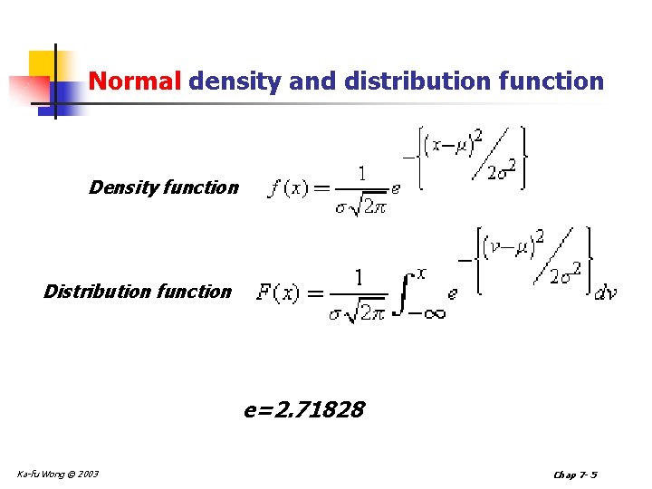
Normal density and distribution function Density function Distribution function e=2. 71828 Ka-fu Wong © 2003 Chap 7 - 5

The density functions of normal distributions with zero mean value and different standard deviations Bell-shaped Symmetric Mean=median = mode Unimodal Asymptotic Ka-fu Wong © 2003 Chap 7 - 6

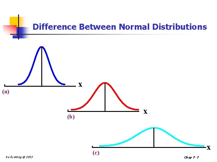
Difference Between Normal Distributions x (a) x (b) Ka-fu Wong © 2003 (c) x Chap 7 - 7

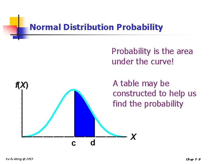
Normal Distribution Probability is the area under the curve! A table may be constructed to help us find the probability f(X) c Ka-fu Wong © 2003 d X Chap 7 - 8

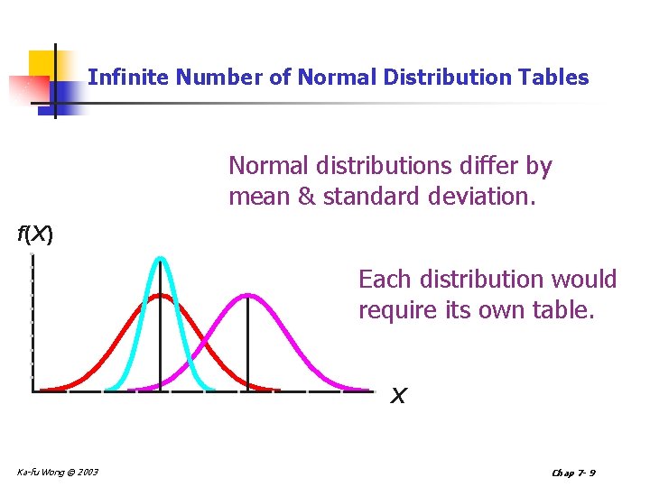
Infinite Number of Normal Distribution Tables Normal distributions differ by mean & standard deviation. f(X) Each distribution would require its own table. X Ka-fu Wong © 2003 Chap 7 - 9

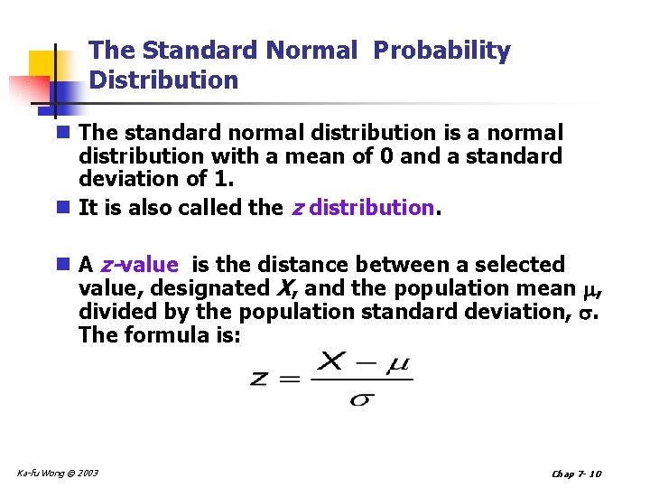
The Standard Normal Probability Distribution n The standard normal distribution is a normal distribution with a mean of 0 and a standard deviation of 1. n It is also called the z distribution. n A z-value is the distance between a selected value, designated X, and the population mean , divided by the population standard deviation, . The formula is: Ka-fu Wong © 2003 Chap 7 - 10

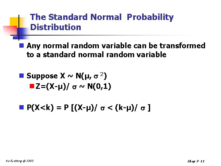
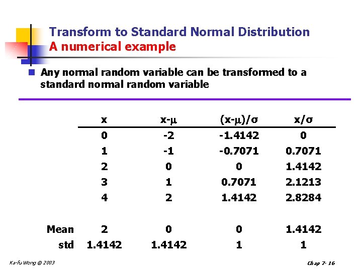
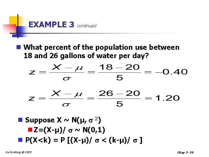
The Standard Normal Probability Distribution n Any normal random variable can be transformed to a standard normal random variable n Suppose X ~ N(µ, 2) n Z=(X-µ)/ ~ N(0, 1) n P(X<k) = P [(X-µ)/ < (k-µ)/ ] Ka-fu Wong © 2003 Chap 7 - 11

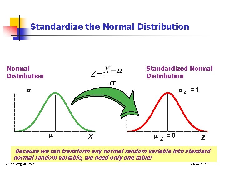
Standardize the Normal Distribution Standardized Normal Distribution z = 1 X Z =0 Z Because we can transform any normal random variable into standard normal random variable, we need only one table! Ka-fu Wong © 2003 Chap 7 - 12

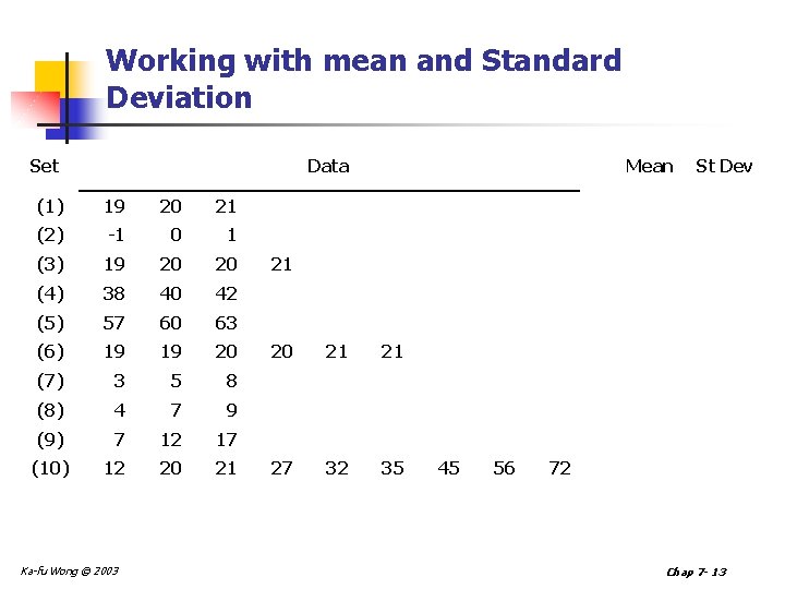
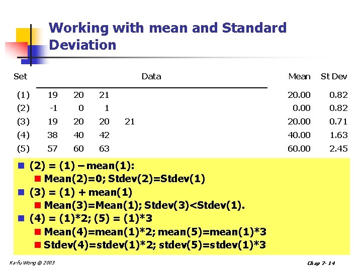
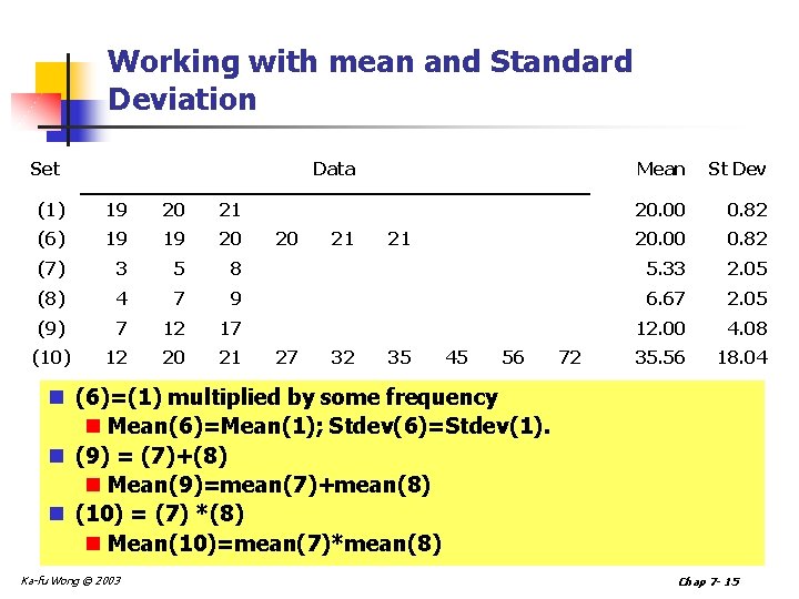
Working with mean and Standard Deviation Set Data Mean St Dev (1) 19 20 21 20. 00 0. 82 (2) -1 0 1 0. 00 0. 82 (3) 19 20 20 20. 00 0. 71 (4) 38 40 42 40. 00 1. 63 (5) 57 60 63 60. 00 2. 45 (6) 19 19 20 20. 00 0. 82 (7) 3 5 8 5. 33 2. 05 (8) 4 7 9 6. 67 2. 05 (9) 7 12 17 12. 00 4. 08 12 20 21 35. 56 18. 04 (10) Ka-fu Wong © 2003 21 20 27 21 32 21 35 45 56 72 Chap 7 - 13

Working with mean and Standard Deviation Set Data Mean St Dev (1) 19 20 21 20. 00 0. 82 (2) -1 0 1 0. 00 0. 82 (3) 19 20 20 20. 00 0. 71 (4) 38 40 42 40. 00 1. 63 (5) 57 60 63 60. 00 2. 45 21 n (2) = (1) – mean(1): n Mean(2)=0; Stdev(2)=Stdev(1) n (3) = (1) + mean(1) n Mean(3)=Mean(1); Stdev(3)<Stdev(1). n (4) = (1)*2; (5) = (1)*3 n Mean(4)=mean(1)*2; mean(5)=mean(1)*3 n Stdev(4)=stdev(1)*2; stdev(5)=stdev(1)*3 Ka-fu Wong © 2003 Chap 7 - 14

Working with mean and Standard Deviation Set Data Mean St Dev 20. 00 0. 82 (1) 19 20 21 (6) 19 19 20 (7) 3 5 8 5. 33 2. 05 (8) 4 7 9 6. 67 2. 05 (9) 7 12 17 12. 00 4. 08 12 20 21 35. 56 18. 04 (10) 20 27 21 32 21 35 45 56 72 n (6)=(1) multiplied by some frequency n Mean(6)=Mean(1); Stdev(6)=Stdev(1). n (9) = (7)+(8) n Mean(9)=mean(7)+mean(8) n (10) = (7) *(8) n Mean(10)=mean(7)*mean(8) Ka-fu Wong © 2003 Chap 7 - 15

Transform to Standard Normal Distribution A numerical example n Any normal random variable can be transformed to a standard normal random variable Mean std Ka-fu Wong © 2003 x x- (x- )/σ x/σ 0 -2 -1. 4142 0 1 -1 -0. 7071 2 0 0 1. 4142 3 1 0. 7071 2. 1213 4 2 1. 4142 2. 8284 2 0 0 1. 4142 1 1 Chap 7 - 16

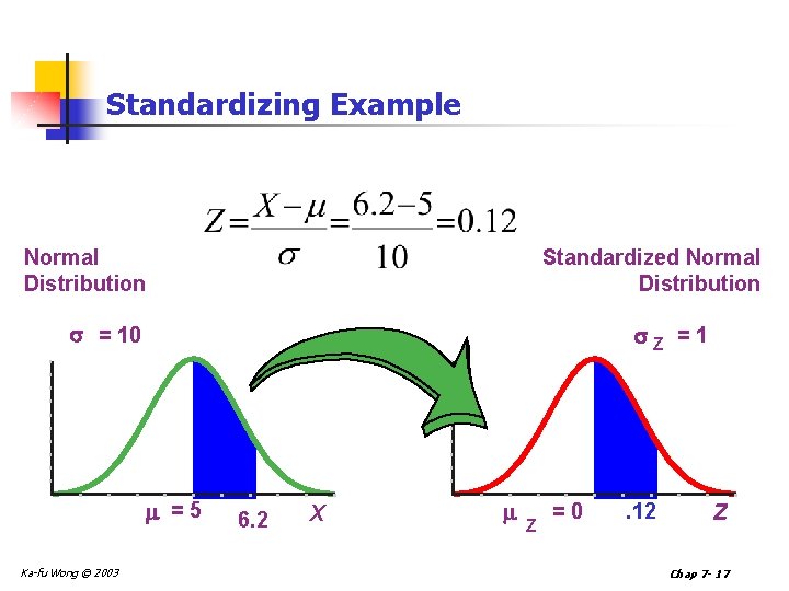
Standardizing Example Normal Distribution Standardized Normal Distribution = 10 Z =1 =5 Ka-fu Wong © 2003 6. 2 X Z =0 . 12 Z Chap 7 - 17

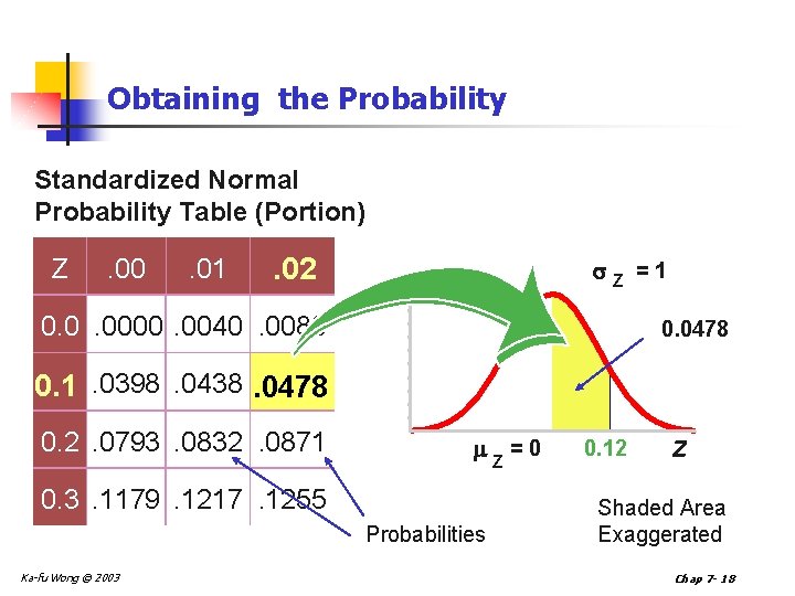
Obtaining the Probability Standardized Normal Probability Table (Portion) Z . 00 . 01 . 02 Z 0. 0. 0000. 0040. 0080 =1 0. 0478 0. 1. 0398. 0438. 0478 0. 2. 0793. 0832. 0871 0. 3. 1179. 1217. 1255 Probabilities Ka-fu Wong © 2003 Z =0 0. 12 Z Shaded Area Exaggerated Chap 7 - 18

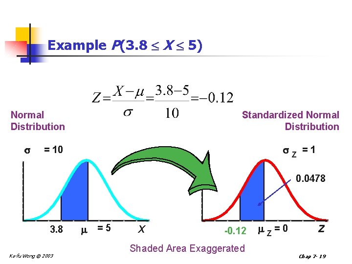
Example P(3. 8 X 5) Normal Distribution Standardized Normal Distribution = 10 Z =1 0. 0478 3. 8 Ka-fu Wong © 2003 =5 X -0. 12 Shaded Area Exaggerated Z =0 Z Chap 7 - 19

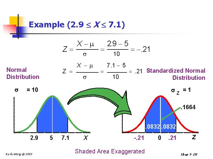
Example (2. 9 X 7. 1) Z Normal Distribution Z X X 2. 9 5 10 7. 1 5 10 . 21 Standardized Normal Distribution = 10 Z =1. 1664 . 0832 2. 9 Ka-fu Wong © 2003 5 7. 1 X -. 21 Shaded Area Exaggerated 0 . 21 Z Chap 7 - 20

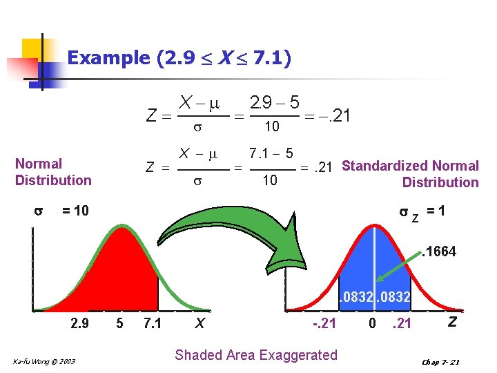
Example (2. 9 X 7. 1) Z Normal Distribution Z X X 2. 9 5 10 7. 1 5 10 . 21 Standardized Normal Distribution = 10 Z =1. 1664 . 0832 2. 9 Ka-fu Wong © 2003 5 7. 1 X -. 21 Shaded Area Exaggerated 0 . 21 Z Chap 7 - 21

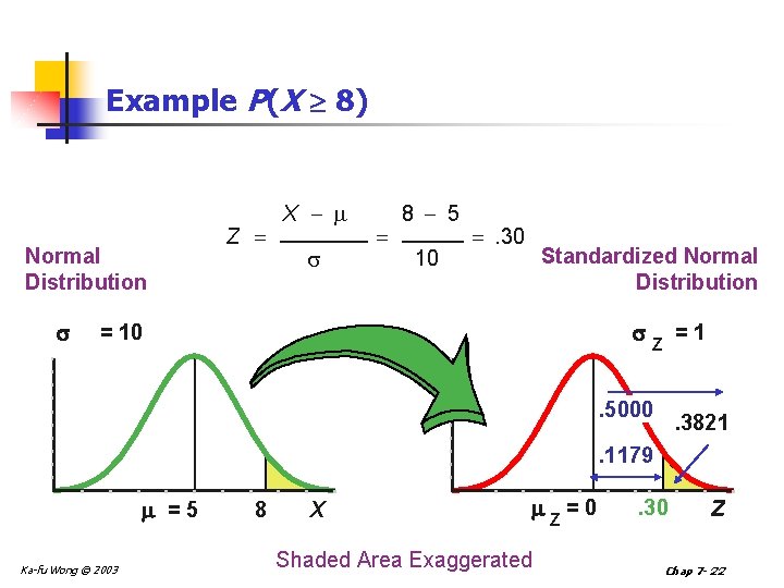
Example P(X 8) Normal Distribution Z X 8 5 10 . 30 Standardized Normal Distribution = 10 =1 Z . 5000 . 3821 . 1179 =5 Ka-fu Wong © 2003 8 X Z=0 Shaded Area Exaggerated . 30 Z Chap 7 - 22

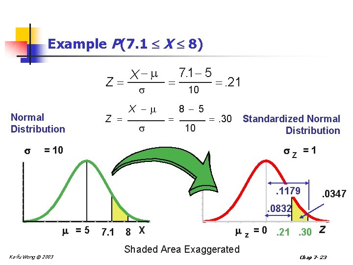
Example P(7. 1 X 8) Z Normal Distribution Z X X 7. 1 5 10 8 5 10 . 21 . 30 Standardized Normal Distribution Z =1 = 10 . 1179 . 0347 . 0832 =5 Ka-fu Wong © 2003 7. 1 8 X Shaded Area Exaggerated z = 0. 21. 30 Z Chap 7 - 23

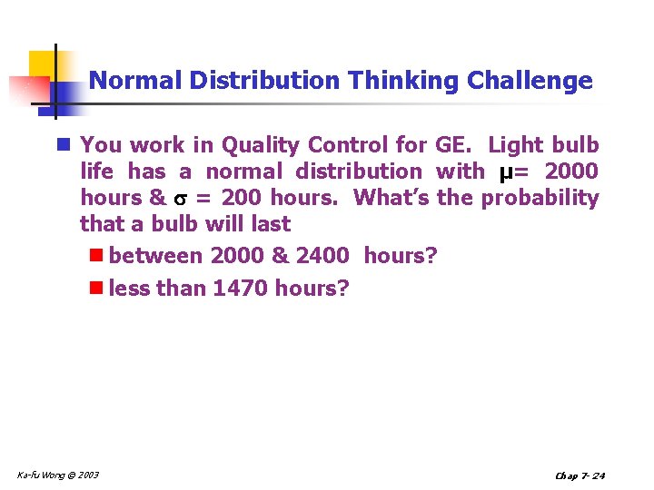
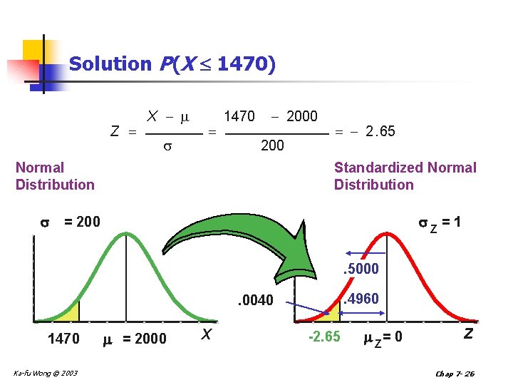
Normal Distribution Thinking Challenge n You work in Quality Control for GE. Light bulb life has a normal distribution with µ= 2000 hours & = 200 hours. What’s the probability that a bulb will last n between 2000 & 2400 hours? n less than 1470 hours? Ka-fu Wong © 2003 Chap 7 - 24

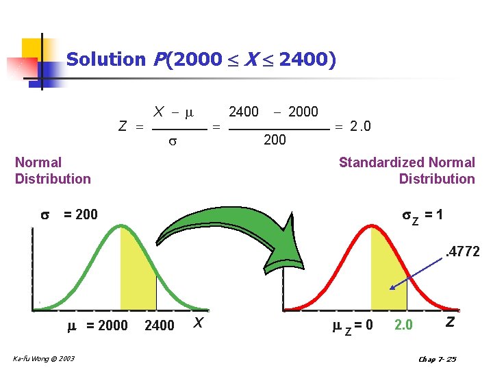
Solution P(2000 X 2400) Z X Normal Distribution 2400 2000 200 2. 0 Standardized Normal Distribution Z = 1 = 200 . 4772 = 2000 Ka-fu Wong © 2003 2400 X Z= 0 2. 0 Z Chap 7 - 25

Solution P(X 1470) Z X 1470 2000 200 Normal Distribution 2. 65 Standardized Normal Distribution Z = 1 = 200. 5000. 4960 . 0040 1470 Ka-fu Wong © 2003 = 2000 X -2. 65 Z= 0 Z Chap 7 - 26

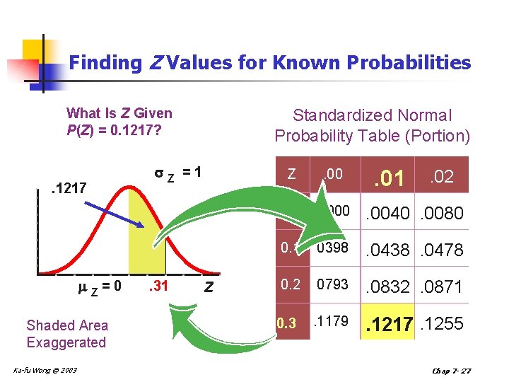
Finding Z Values for Known Probabilities What Is Z Given P(Z) = 0. 1217? . 1217 Z =0 Shaded Area Exaggerated Ka-fu Wong © 2003 Z . 31 Standardized Normal Probability Table (Portion) =1 Z . 00 0. 0 . 0000 . 0040. 0080 0. 1. 0398 . 0438. 0478 0. 2. 0793 . 0832. 0871 . 1179 . 1217. 1255 0. 3 . 02 Chap 7 - 27

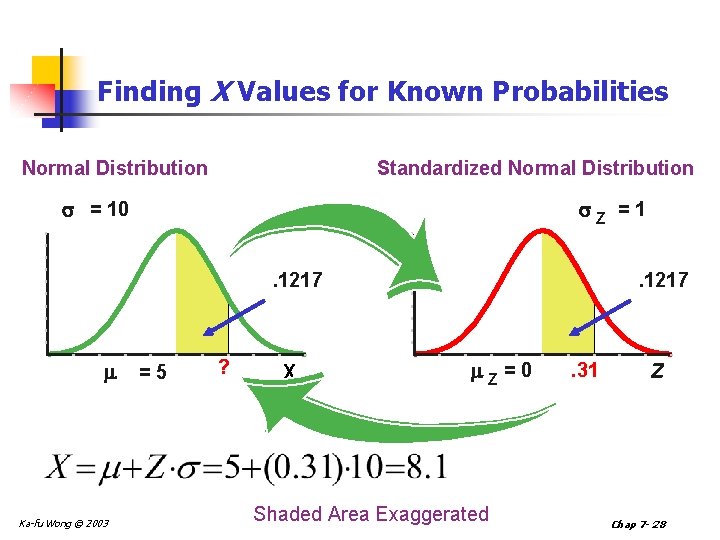
Finding X Values for Known Probabilities Normal Distribution Standardized Normal Distribution = 10 Z =1. 1217 Ka-fu Wong © 2003 =5 ? X . 1217 Z =0 Shaded Area Exaggerated . 31 Z Chap 7 - 28

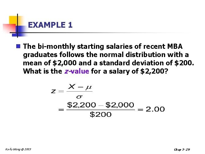
EXAMPLE 1 n The bi-monthly starting salaries of recent MBA graduates follows the normal distribution with a mean of $2, 000 and a standard deviation of $200. What is the z-value for a salary of $2, 200? Ka-fu Wong © 2003 Chap 7 - 29

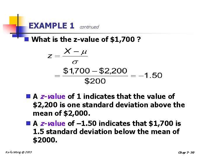
EXAMPLE 1 continued n What is the z-value of $1, 700 ? n A z-value of 1 indicates that the value of $2, 200 is one standard deviation above the mean of $2, 000. n A z-value of – 1. 50 indicates that $1, 700 is 1. 5 standard deviation below the mean of $2000. Ka-fu Wong © 2003 Chap 7 - 30

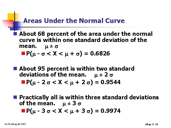
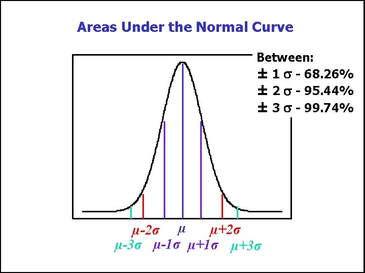
Areas Under the Normal Curve n About 68 percent of the area under the normal curve is within one standard deviation of the mean. ± n P( - < X < + ) = 0. 6826 n About 95 percent is within two standard deviations of the mean. ± 2 n P( - 2 < X < + 2 ) = 0. 9544 n Practically all is within three standard deviations of the mean. ± 3 n P( - 3 < X < + 3 ) = 0. 9974 Ka-fu Wong © 2003 Chap 7 - 31

Areas Under the Normal Curve Between: ± 1 - 68. 26% ± 2 - 95. 44% ± 3 - 99. 74% µ+2σ µ-2σ µ µ-3σ µ-1σ µ+3σ Ka-fu Wong © 2003 Chap 7 - 32

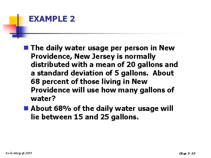
EXAMPLE 2 n The daily water usage person in New Providence, New Jersey is normally distributed with a mean of 20 gallons and a standard deviation of 5 gallons. About 68 percent of those living in New Providence will use how many gallons of water? n About 68% of the daily water usage will lie between 15 and 25 gallons. Ka-fu Wong © 2003 Chap 7 - 33

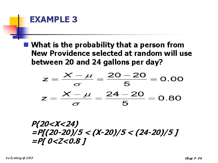
EXAMPLE 3 n What is the probability that a person from New Providence selected at random will use between 20 and 24 gallons per day? P(20<X<24) =P[(20 -20)/5 < (X-20)/5 < (24 -20)/5 ] =P[ 0<Z<0. 8 ] Ka-fu Wong © 2003 Chap 7 - 34

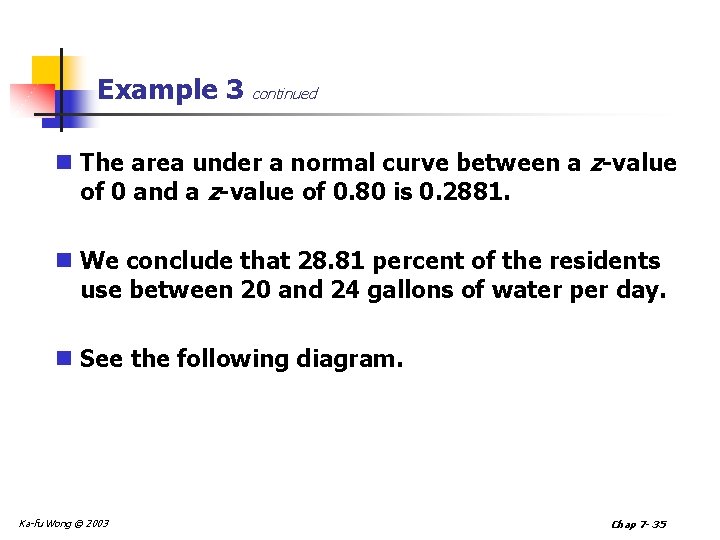
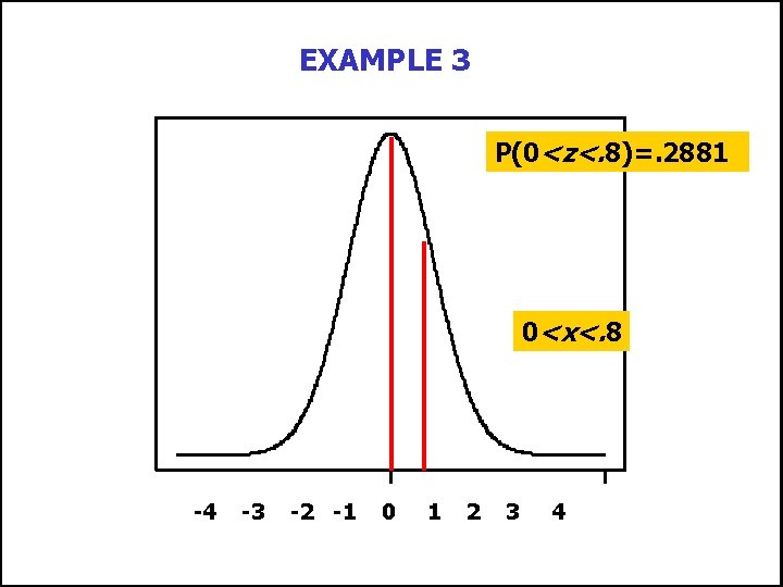
Example 3 continued n The area under a normal curve between a z-value of 0 and a z-value of 0. 80 is 0. 2881. n We conclude that 28. 81 percent of the residents use between 20 and 24 gallons of water per day. n See the following diagram. Ka-fu Wong © 2003 Chap 7 - 35

EXAMPLE 3 P(0<z<. 8)=. 2881 0<x<. 8 -4 Ka-fu Wong © 2003 -3 -2 -1 x 0 1 2 3 4 Chap 7 - 36

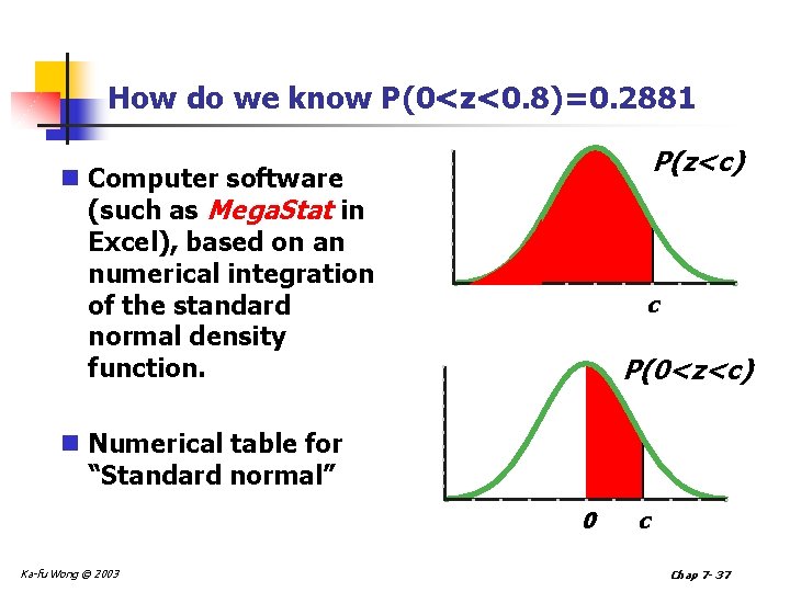
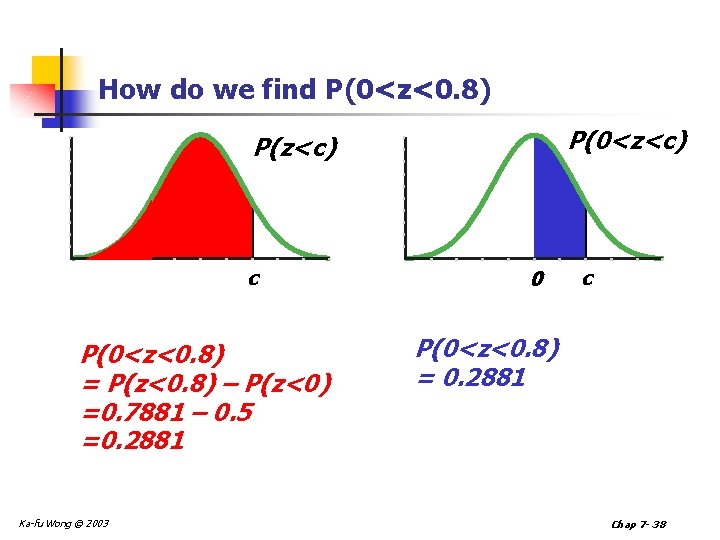
How do we know P(0<z<0. 8)=0. 2881 P(z<c) n Computer software (such as Mega. Stat in Excel), based on an numerical integration of the standard normal density function. c P(0<z<c) n Numerical table for “Standard normal” 0 Ka-fu Wong © 2003 c Chap 7 - 37

How do we find P(0<z<0. 8) P(0<z<c) P(z<c) c P(0<z<0. 8) = P(z<0. 8) – P(z<0) =0. 7881 – 0. 5 =0. 2881 Ka-fu Wong © 2003 0 c P(0<z<0. 8) = 0. 2881 Chap 7 - 38

EXAMPLE 3 continued n What percent of the population use between 18 and 26 gallons of water per day? n Suppose X ~ N(µ, 2) n Z=(X-µ)/ ~ N(0, 1) n P(X<k) = P [(X-µ)/ < (k-µ)/ ] Ka-fu Wong © 2003 Chap 7 - 39

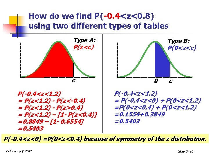
How do we find P(-0. 4<z<0. 8) using two different types of tables Type A: P(z<c) c P(-0. 4<z<1. 2) = P(z<1. 2) - P(z<-0. 4) = P(z<1. 2) - P(z>0. 4) = P(z<1. 2) – [1 - P(z<0. 4)] =0. 8849 – [1 - 0. 6554] =0. 5403 Type B: P(0<z<c) 0 c P(-0. 4<z<1. 2) = P(-0. 4<z<0) + P(0<z<1. 2) =P(0<z<0. 4) + P(0<z<1. 2) =0. 1554+0. 3849 =0. 5403 P(-0. 4<z<0) =P(0<z<0. 4) because of symmetry of the z distribution. Ka-fu Wong © 2003 Chap 7 - 40

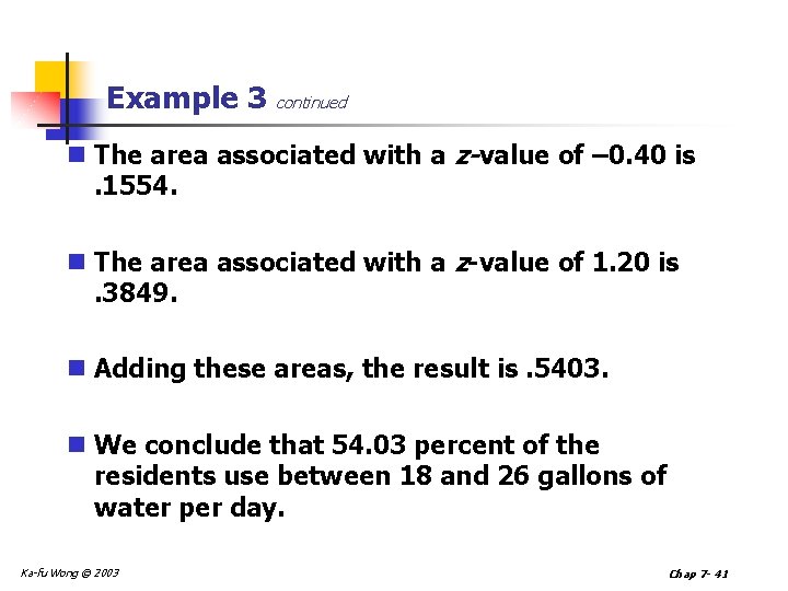
Example 3 continued n The area associated with a z-value of – 0. 40 is. 1554. n The area associated with a z-value of 1. 20 is. 3849. n Adding these areas, the result is. 5403. n We conclude that 54. 03 percent of the residents use between 18 and 26 gallons of water per day. Ka-fu Wong © 2003 Chap 7 - 41

EXAMPLE 4 n Professor Mann has determined that the scores in his statistics course are approximately normally distributed with a mean of 72 and a standard deviation of 5. He announces to the class that the top 15 percent of the scores will earn an A. What is the lowest score a student can earn and still receive an A? Ka-fu Wong © 2003 Chap 7 - 42

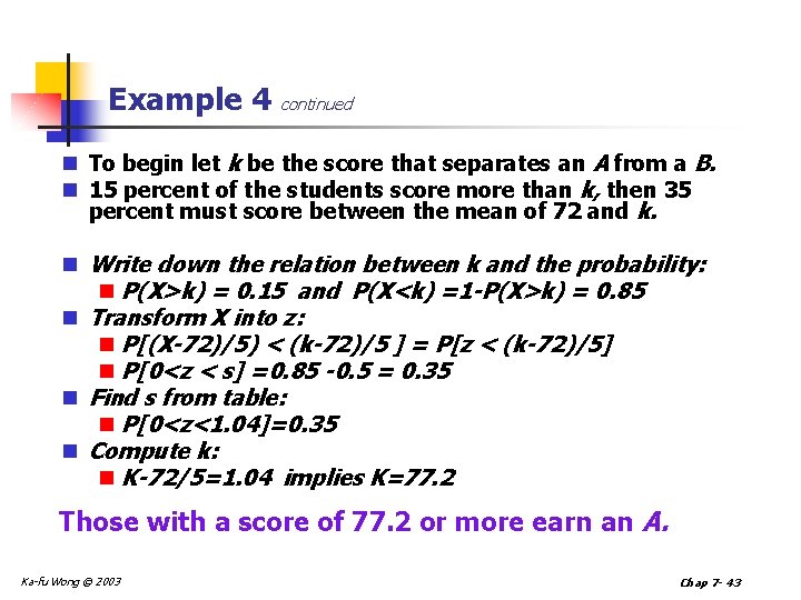
Example 4 continued n To begin let k be the score that separates an A from a B. n 15 percent of the students score more than k, then 35 percent must score between the mean of 72 and k. n Write down the relation between k and the probability: n P(X>k) = 0. 15 and P(X<k) =1 -P(X>k) = 0. 85 n Transform X into z: n P[(X-72)/5) < (k-72)/5 ] = P[z < (k-72)/5] n P[0<z < s] =0. 85 -0. 5 = 0. 35 n Find s from table: n P[0<z<1. 04]=0. 35 n Compute k: n K-72/5=1. 04 implies K=77. 2 Those with a score of 77. 2 or more earn an A. Ka-fu Wong © 2003 Chap 7 - 43

The Normal Approximation to the Binomial n The normal distribution (a continuous distribution) yields a good approximation of the binomial distribution (a discrete distribution) for large values of n. n The normal probability distribution is generally a good approximation to the binomial probability distribution when n and n(1 - ) are both greater than 5. Ka-fu Wong © 2003 Chap 7 - 44

The Normal Approximation continued Recall for the binomial experiment: n There are only two mutually exclusive outcomes (success or failure) on each trial. n A binomial distribution results from counting the number of successes. n Each trial is independent. n The probability is fixed from trial to trial, and the number of trials n is also fixed. Ka-fu Wong © 2003 Chap 7 - 45

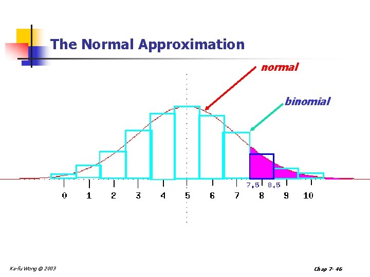
The Normal Approximation normal binomial Ka-fu Wong © 2003 Chap 7 - 46

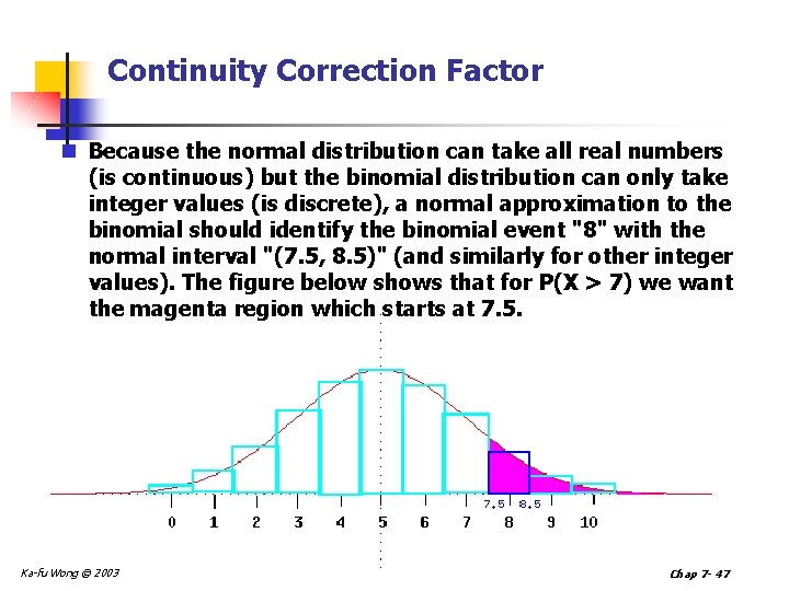
Continuity Correction Factor n Because the normal distribution can take all real numbers (is continuous) but the binomial distribution can only take integer values (is discrete), a normal approximation to the binomial should identify the binomial event "8" with the normal interval "(7. 5, 8. 5)" (and similarly for other integer values). The figure below shows that for P(X > 7) we want the magenta region which starts at 7. 5. Ka-fu Wong © 2003 Chap 7 - 47

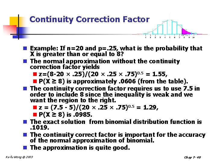
Continuity Correction Factor n Example: If n=20 and p=. 25, what is the probability that X is greater than or equal to 8? n The normal approximation without the continuity correction factor yields n z=(8 -20 ×. 25)/(20 ×. 25 ×. 75)0. 5 = 1. 55, n P(X ≥ 8) is approximately. 0606 (from the table). n The continuity correction factor requires us to use 7. 5 in order to include 8 since the inequality is weak and we want the region to the right. n z = (7. 5 - 5)/(20 ×. 25 ×. 75)0. 5 = 1. 29, n P(X ≥ 8) is. 0985. n The exact solution from binomial distribution function is. 1019. n The continuity correct factor is important for the accuracy of the normal approximation of binomial. n The approximation is quite good. Ka-fu Wong © 2003 Chap 7 - 48

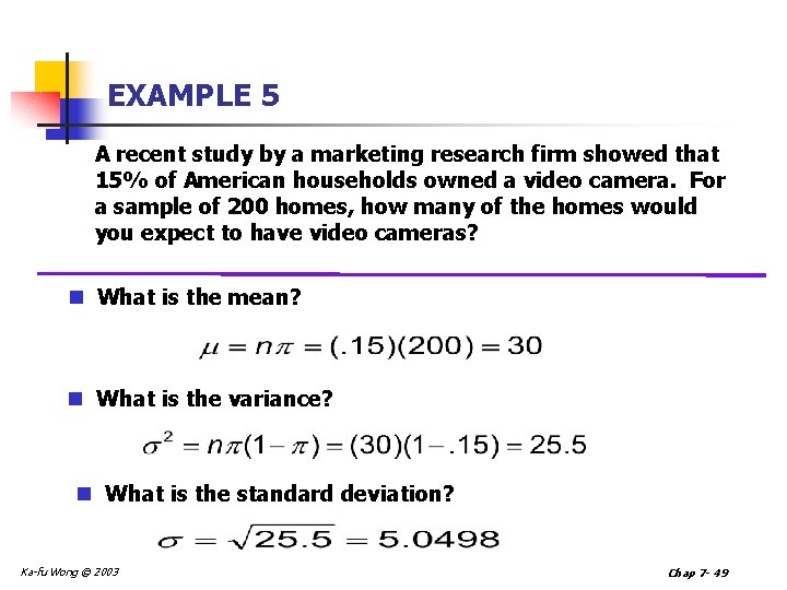
EXAMPLE 5 A recent study by a marketing research firm showed that 15% of American households owned a video camera. For a sample of 200 homes, how many of the homes would you expect to have video cameras? n What is the mean? n What is the variance? n What is the standard deviation? Ka-fu Wong © 2003 Chap 7 - 49

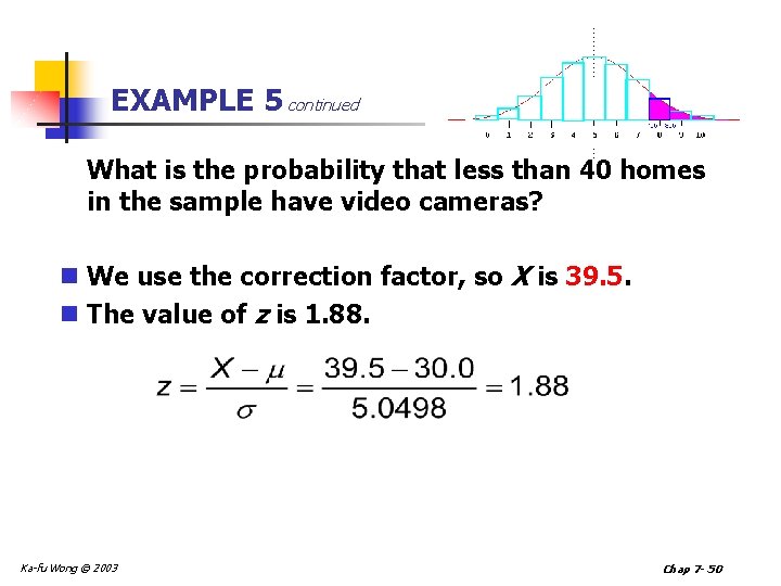
EXAMPLE 5 continued What is the probability that less than 40 homes in the sample have video cameras? n We use the correction factor, so X is 39. 5. n The value of z is 1. 88. Ka-fu Wong © 2003 Chap 7 - 50

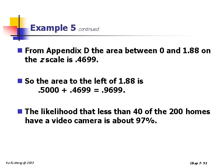
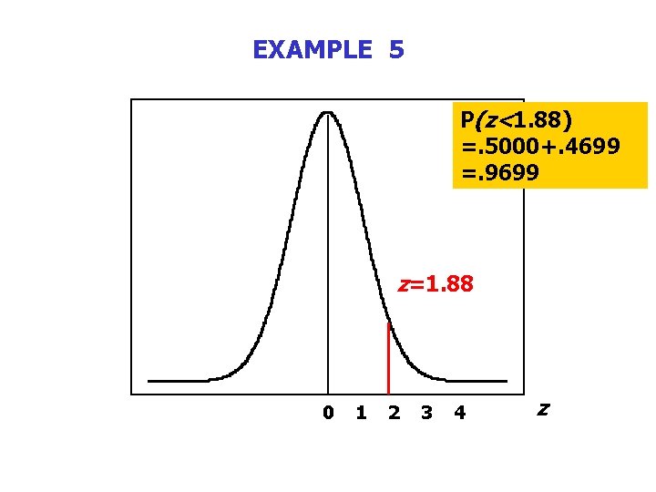
Example 5 continued n From Appendix D the area between 0 and 1. 88 on the z scale is. 4699. n So the area to the left of 1. 88 is. 5000 +. 4699 =. 9699. n The likelihood that less than 40 of the 200 homes have a video camera is about 97%. Ka-fu Wong © 2003 Chap 7 - 51

EXAMPLE 5 P(z<1. 88) =. 5000+. 4699 =. 9699 z=1. 88 0 Ka-fu Wong © 2003 1 2 3 4 z Chap 7 - 52

Chapter Seven The Normal Probability Distribution - END - Ka-fu Wong © 2003 Chap 7 - 53