Dr Kafu Wong ECON 1003 Analysis of Economic

Dr. Ka-fu Wong ECON 1003 Analysis of Economic Data Ka-fu Wong © 2003 Chap 6 - 1

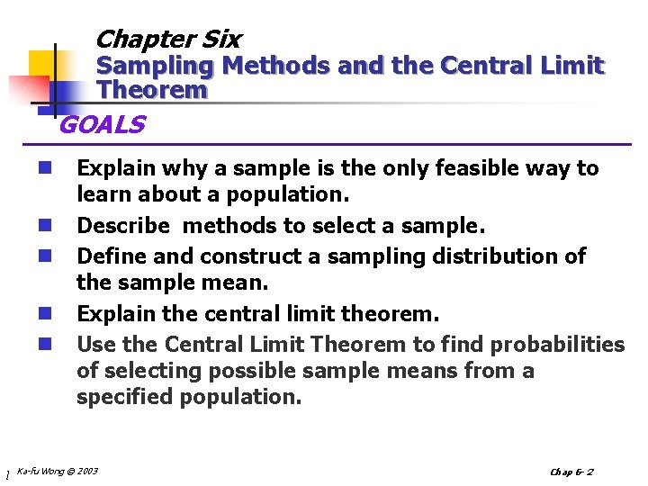
Chapter Six Sampling Methods and the Central Limit Theorem GOALS n n n l Explain why a sample is the only feasible way to learn about a population. Describe methods to select a sample. Define and construct a sampling distribution of the sample mean. Explain the central limit theorem. Use the Central Limit Theorem to find probabilities of selecting possible sample means from a specified population. Ka-fu Wong © 2003 Chap 6 - 2

Why Sample the Population? n The physical impossibility of checking all items in the population. n The cost of studying all the items in a population. n The sample results are usually adequate. n Contacting the whole population would often be time-consuming. n The destructive nature of certain tests. Ka-fu Wong © 2003 Chap 6 - 3

Probability Sampling n A probability sample is a sample selected such that each item or person in the population being studied has a known likelihood of being included in the sample. Ka-fu Wong © 2003 Chap 6 - 4

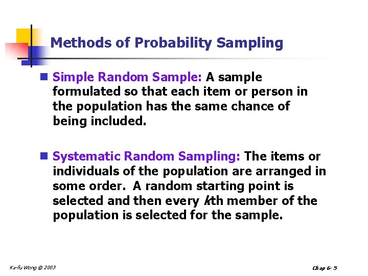
Methods of Probability Sampling n Simple Random Sample: A sample formulated so that each item or person in the population has the same chance of being included. n Systematic Random Sampling: The items or individuals of the population are arranged in some order. A random starting point is selected and then every kth member of the population is selected for the sample. Ka-fu Wong © 2003 Chap 6 - 5

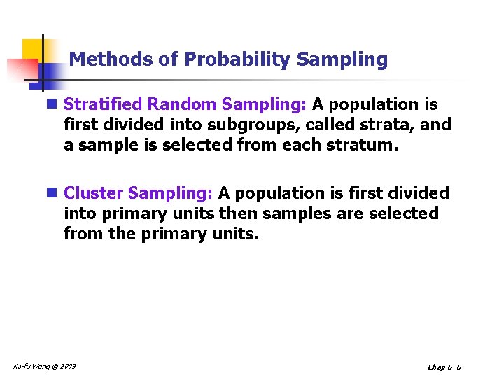
Methods of Probability Sampling n Stratified Random Sampling: A population is first divided into subgroups, called strata, and a sample is selected from each stratum. n Cluster Sampling: A population is first divided into primary units then samples are selected from the primary units. Ka-fu Wong © 2003 Chap 6 - 6

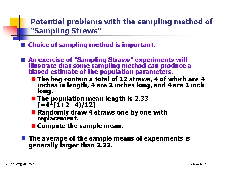
Potential problems with the sampling method of “Sampling Straws” n Choice of sampling method is important. n An exercise of “Sampling Straws” experiments will illustrate that some sampling method can produce a biased estimate of the population parameters. n The bag contain a total of 12 straws, 4 of which are 4 inches in length, 4 are 2 inches long, and 4 are 1 inch long. n The population mean length is 2. 33 (=4*(1+2+4)/12) n Randomly draw 4 straws one by one with replacement. n Compute the sample mean. n The average of the sample means of experiments is generally larger than 2. 33. Ka-fu Wong © 2003 Chap 6 - 7

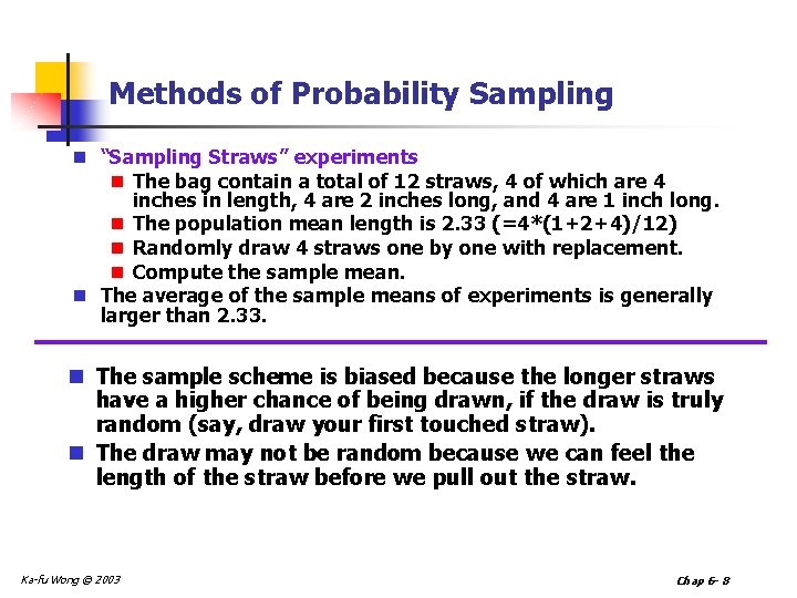
Methods of Probability Sampling n “Sampling Straws” experiments n The bag contain a total of 12 straws, 4 of which are 4 inches in length, 4 are 2 inches long, and 4 are 1 inch long. n The population mean length is 2. 33 (=4*(1+2+4)/12) n Randomly draw 4 straws one by one with replacement. n Compute the sample mean. n The average of the sample means of experiments is generally larger than 2. 33. n The sample scheme is biased because the longer straws have a higher chance of being drawn, if the draw is truly random (say, draw your first touched straw). n The draw may not be random because we can feel the length of the straw before we pull out the straw. Ka-fu Wong © 2003 Chap 6 - 8

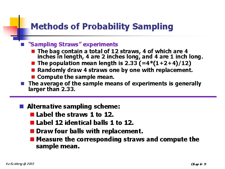
Methods of Probability Sampling n “Sampling Straws” experiments n The bag contain a total of 12 straws, 4 of which are 4 inches in length, 4 are 2 inches long, and 4 are 1 inch long. n The population mean length is 2. 33 (=4*(1+2+4)/12) n Randomly draw 4 straws one by one with replacement. n Compute the sample mean. n The average of the sample means of experiments is generally larger than 2. 33. n Alternative sampling scheme: n Label the straws 1 to 12. n Label 12 identical balls 1 to 12. n Draw four balls with replacement. n Measure the corresponding straws and compute the sample mean. Ka-fu Wong © 2003 Chap 6 - 9

Methods of Probability Sampling n In nonprobability sample, whether an observation is included in the sample is based on the judgment of the person selecting the sample. n The sampling error is the difference between a sample statistic and its corresponding population parameter. n Sampling error is almost always nonzero. Ka-fu Wong © 2003 Chap 6 - 10

Sampling Distribution of the Sample Means n The sampling distribution of the sample mean is a probability distribution consisting of all possible sample means of a given sample size selected from a population. Ka-fu Wong © 2003 Chap 6 - 11

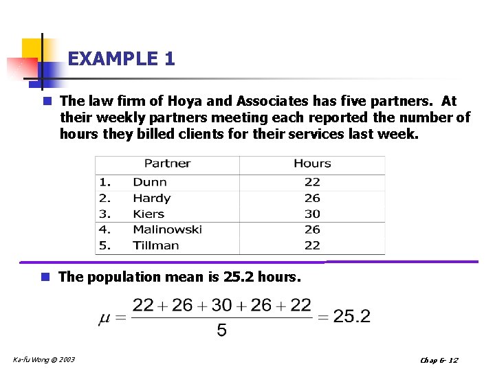
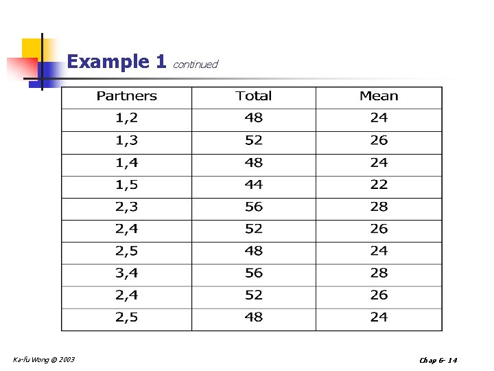
EXAMPLE 1 n The law firm of Hoya and Associates has five partners. At their weekly partners meeting each reported the number of hours they billed clients for their services last week. n The population mean is 25. 2 hours. Ka-fu Wong © 2003 Chap 6 - 12

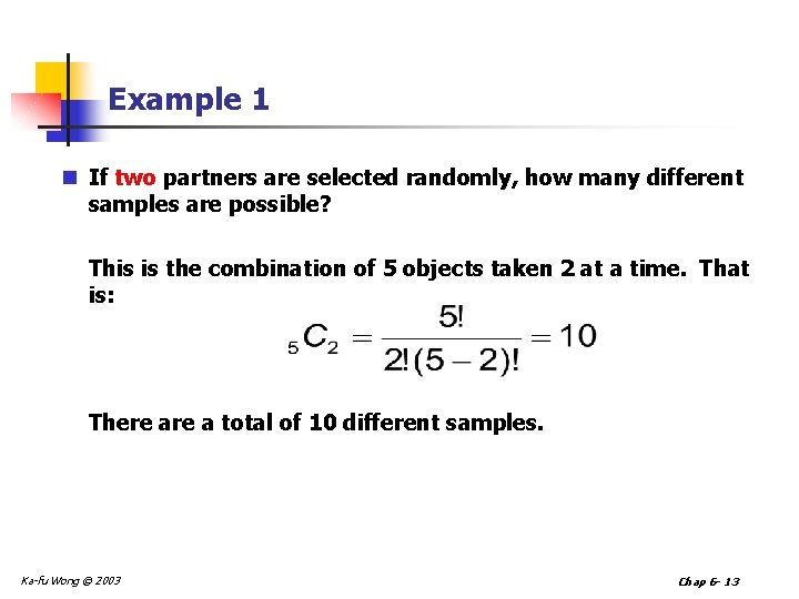
Example 1 n If two partners are selected randomly, how many different samples are possible? This is the combination of 5 objects taken 2 at a time. That is: There a total of 10 different samples. Ka-fu Wong © 2003 Chap 6 - 13

Example 1 continued Ka-fu Wong © 2003 Chap 6 - 14

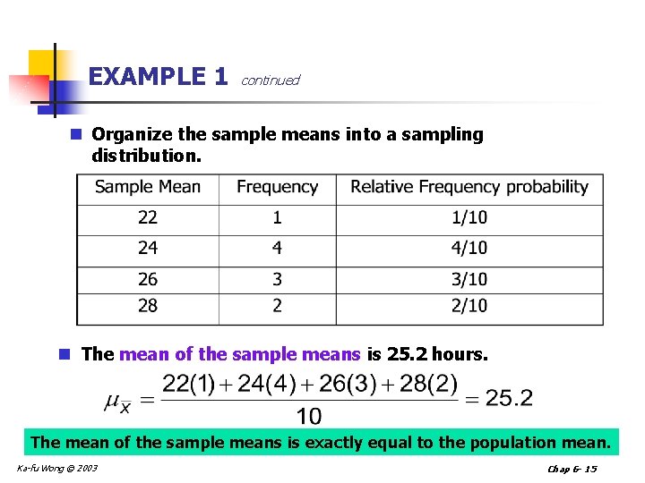
EXAMPLE 1 continued n Organize the sample means into a sampling distribution. n The mean of the sample means is 25. 2 hours. The mean of the sample means is exactly equal to the population mean. Ka-fu Wong © 2003 Chap 6 - 15

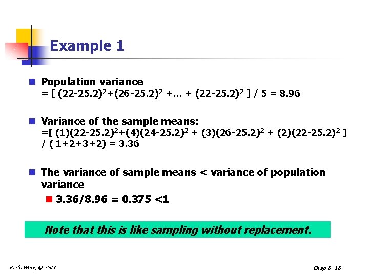
Example 1 n Population variance = [ (22 -25. 2)2+(26 -25. 2)2 +… + (22 -25. 2)2 ] / 5 = 8. 96 n Variance of the sample means: =[ (1)(22 -25. 2)2+(4)(24 -25. 2)2 + (3)(26 -25. 2)2 + (2)(22 -25. 2)2 ] / ( 1+2+3+2) = 3. 36 n The variance of sample means < variance of population variance n 3. 36/8. 96 = 0. 375 <1 Note that this is like sampling without replacement. Ka-fu Wong © 2003 Chap 6 - 16

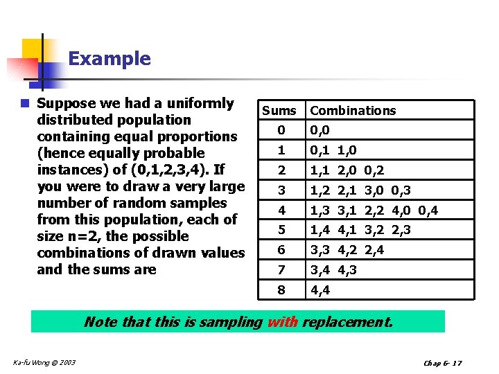
Example n Suppose we had a uniformly distributed population containing equal proportions (hence equally probable instances) of (0, 1, 2, 3, 4). If you were to draw a very large number of random samples from this population, each of size n=2, the possible combinations of drawn values and the sums are Sums Combinations 0 0, 0 1 0, 1 1, 0 2 1, 1 2, 0 0, 2 3 1, 2 2, 1 3, 0 0, 3 4 1, 3 3, 1 2, 2 4, 0 0, 4 5 1, 4 4, 1 3, 2 2, 3 6 3, 3 4, 2 2, 4 7 3, 4 4, 3 8 4, 4 Note that this is sampling with replacement. Ka-fu Wong © 2003 Chap 6 - 17

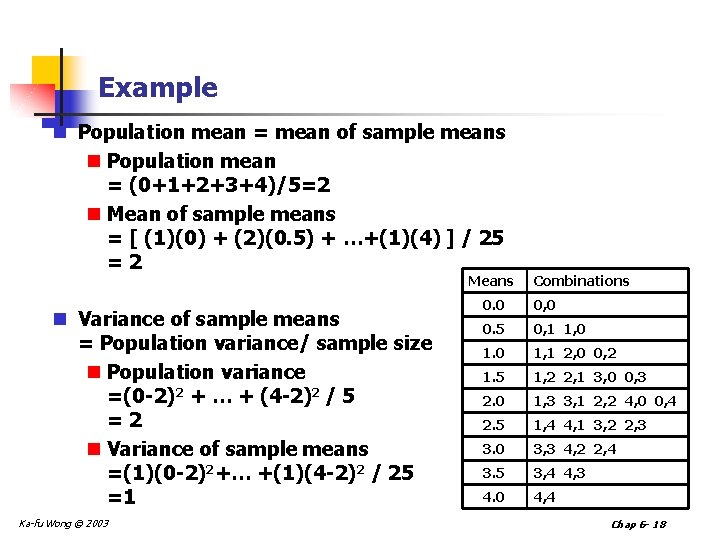
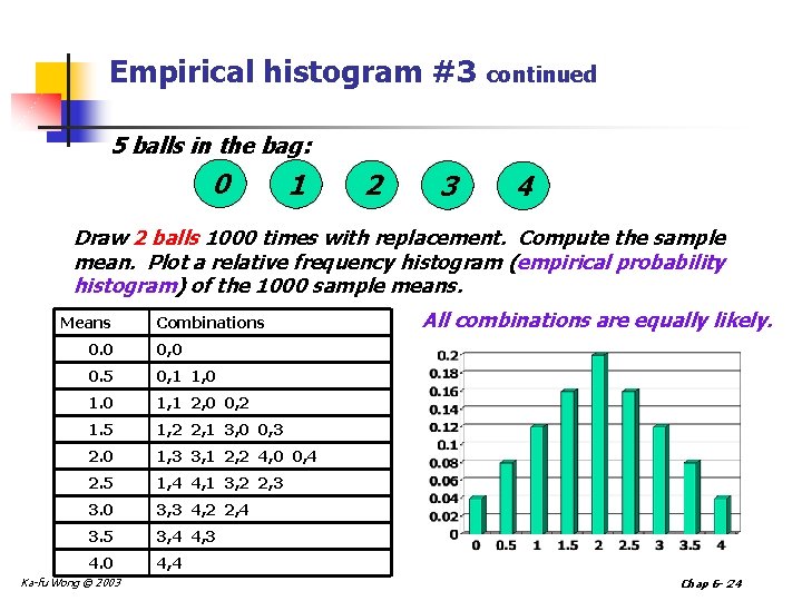
Example n Population mean = mean of sample means n Population mean = (0+1+2+3+4)/5=2 n Mean of sample means = [ (1)(0) + (2)(0. 5) + …+(1)(4) ] / 25 =2 Means n Variance of sample means = Population variance/ sample size n Population variance =(0 -2)2 + … + (4 -2)2 / 5 =2 n Variance of sample means =(1)(0 -2)2+… +(1)(4 -2)2 / 25 =1 Ka-fu Wong © 2003 Combinations 0. 0 0, 0 0. 5 0, 1 1, 0 1, 1 2, 0 0, 2 1. 5 1, 2 2, 1 3, 0 0, 3 2. 0 1, 3 3, 1 2, 2 4, 0 0, 4 2. 5 1, 4 4, 1 3, 2 2, 3 3. 0 3, 3 4, 2 2, 4 3. 5 3, 4 4, 3 4. 0 4, 4 Chap 6 - 18

Probability Histograms n In a probability histograms, the area of the bar represents the chance of a value happening as a result of the random (chance) process n Empirical histograms (from observed data) for a process converge to the probability histogram Ka-fu Wong © 2003 Chap 6 - 19

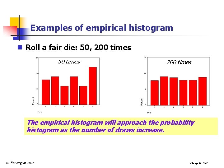
Examples of empirical histogram n Roll a fair die: 50, 200 times 50 times 200 times The empirical histogram will approach the probability histogram as the number of draws increase. Ka-fu Wong © 2003 Chap 6 - 20

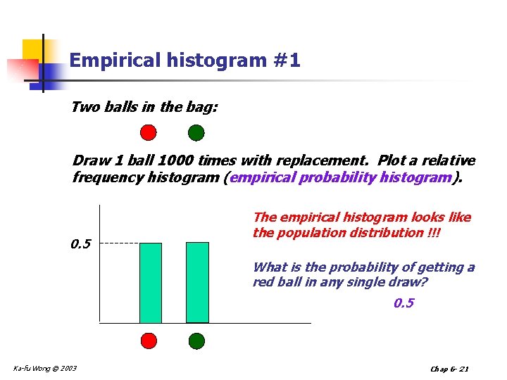
Empirical histogram #1 Two balls in the bag: Draw 1 ball 1000 times with replacement. Plot a relative frequency histogram (empirical probability histogram). 0. 5 The empirical histogram looks like the population distribution !!! What is the probability of getting a red ball in any single draw? 0. 5 Ka-fu Wong © 2003 Chap 6 - 21

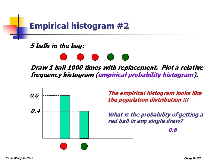
Empirical histogram #2 5 balls in the bag: Draw 1 ball 1000 times with replacement. Plot a relative frequency histogram (empirical probability histogram). 0. 6 0. 4 The empirical histogram looks like the population distribution !!! What is the probability of getting a red ball in any single draw? 0. 6 Ka-fu Wong © 2003 Chap 6 - 22

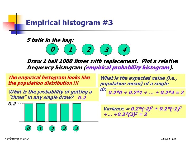
Empirical histogram #3 5 balls in the bag: 0 1 2 3 4 Draw 1 ball 1000 times with replacement. Plot a relative frequency histogram (empirical probability histogram). The empirical histogram looks like the population distribution !!! What is the probability of getting a “three” in any single draw? 0. 2 0 Ka-fu Wong © 2003 1 2 3 What is the expected value (i. e. , population mean) of a single draw? 0. 2*0 + 0. 2*1 + … + 0. 2*4 = 2 Variance = 0. 2*(-2)2 + 0. 2*(-1)2 +… +0. 2*(2)2 = 2 4 Chap 6 - 23

Empirical histogram #3 continued 5 balls in the bag: 0 1 2 3 4 Draw 2 balls 1000 times with replacement. Compute the sample mean. Plot a relative frequency histogram (empirical probability histogram) of the 1000 sample means. Means Combinations 0. 0 0, 0 0. 5 0, 1 1, 0 1, 1 2, 0 0, 2 1. 5 1, 2 2, 1 3, 0 0, 3 2. 0 1, 3 3, 1 2, 2 4, 0 0, 4 2. 5 1, 4 4, 1 3, 2 2, 3 3. 0 3, 3 4, 2 2, 4 3. 5 3, 4 4, 3 4. 0 4, 4 Ka-fu Wong © 2003 All combinations are equally likely. Chap 6 - 24

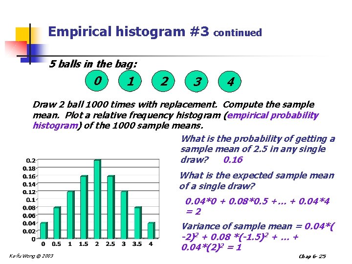
Empirical histogram #3 continued 5 balls in the bag: 0 1 2 3 4 Draw 2 ball 1000 times with replacement. Compute the sample mean. Plot a relative frequency histogram (empirical probability histogram) of the 1000 sample means. What is the probability of getting a sample mean of 2. 5 in any single draw? 0. 16 What is the expected sample mean of a single draw? 0. 04*0 + 0. 08*0. 5 +… + 0. 04*4 =2 Variance of sample mean = 0. 04*( -2)2 + 0. 08 *(-1. 5)2 + … + 0. 04*(2)2 = 1 Ka-fu Wong © 2003 Chap 6 - 25

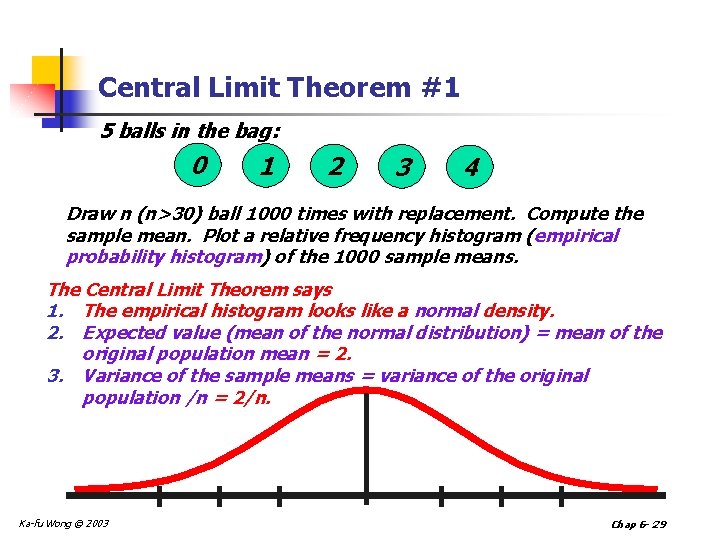
Central Limit Theorem #1 5 balls in the bag: 0 1 2 3 4 Draw n (n>30) ball 1000 times with replacement. Compute the sample mean. Plot a relative frequency histogram (empirical probability histogram) of the 1000 sample means. The Central Limit Theorem says 1. The empirical histogram looks like a normal density. 2. Expected value (mean of the normal distribution) = mean of the original population mean = 2. 3. Variance of the sample means = variance of the original population /n = 2/n. Ka-fu Wong © 2003 Chap 6 - 29

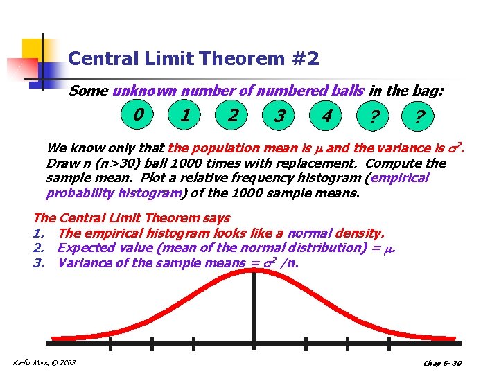
Central Limit Theorem #2 Some unknown number of numbered balls in the bag: 0 1 2 3 4 ? ? We know only that the population mean is and the variance is 2. Draw n (n>30) ball 1000 times with replacement. Compute the sample mean. Plot a relative frequency histogram (empirical probability histogram) of the 1000 sample means. The Central Limit Theorem says 1. The empirical histogram looks like a normal density. 2. Expected value (mean of the normal distribution) = . 3. Variance of the sample means = 2 /n. Ka-fu Wong © 2003 Chap 6 - 30

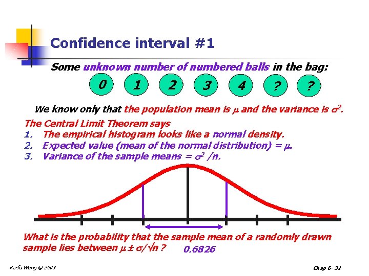
Confidence interval #1 Some unknown number of numbered balls in the bag: 0 1 2 3 4 ? ? We know only that the population mean is and the variance is 2. The Central Limit Theorem says 1. The empirical histogram looks like a normal density. 2. Expected value (mean of the normal distribution) = . 3. Variance of the sample means = 2 /n. What is the probability that the sample mean of a randomly drawn sample lies between / n ? 0. 6826 Ka-fu Wong © 2003 Chap 6 - 31

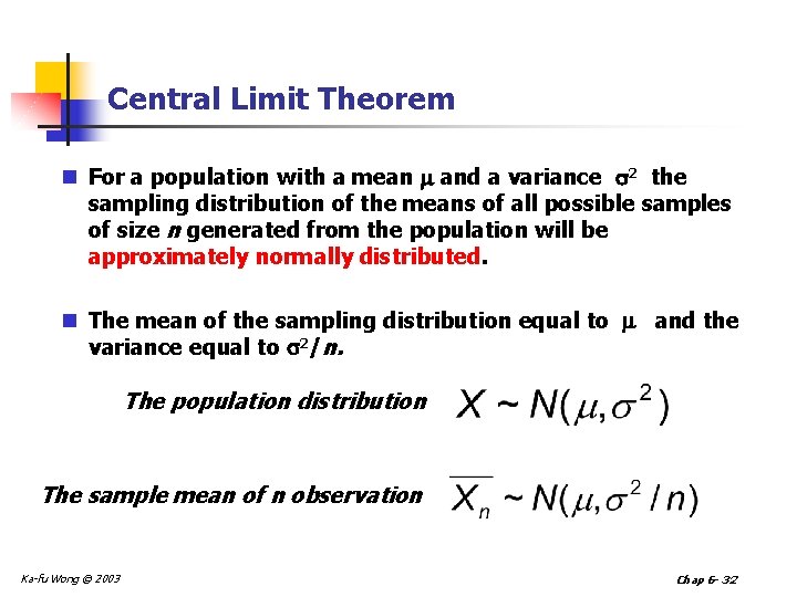
Central Limit Theorem n For a population with a mean and a variance 2 the sampling distribution of the means of all possible samples of size n generated from the population will be approximately normally distributed. n The mean of the sampling distribution equal to and the variance equal to 2/n. The population distribution The sample mean of n observation Ka-fu Wong © 2003 Chap 6 - 32

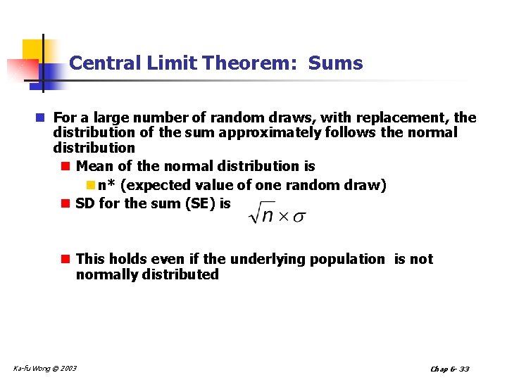
Central Limit Theorem: Sums n For a large number of random draws, with replacement, the distribution of the sum approximately follows the normal distribution n Mean of the normal distribution is n n* (expected value of one random draw) n SD for the sum (SE) is n This holds even if the underlying population is not normally distributed Ka-fu Wong © 2003 Chap 6 - 33

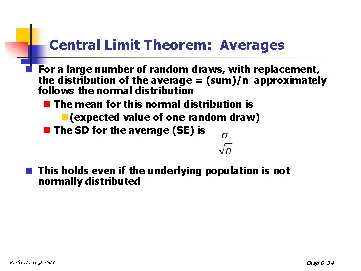
Central Limit Theorem: Averages n For a large number of random draws, with replacement, the distribution of the average = (sum)/n approximately follows the normal distribution n The mean for this normal distribution is n (expected value of one random draw) n The SD for the average (SE) is n This holds even if the underlying population is not normally distributed Ka-fu Wong © 2003 Chap 6 - 34

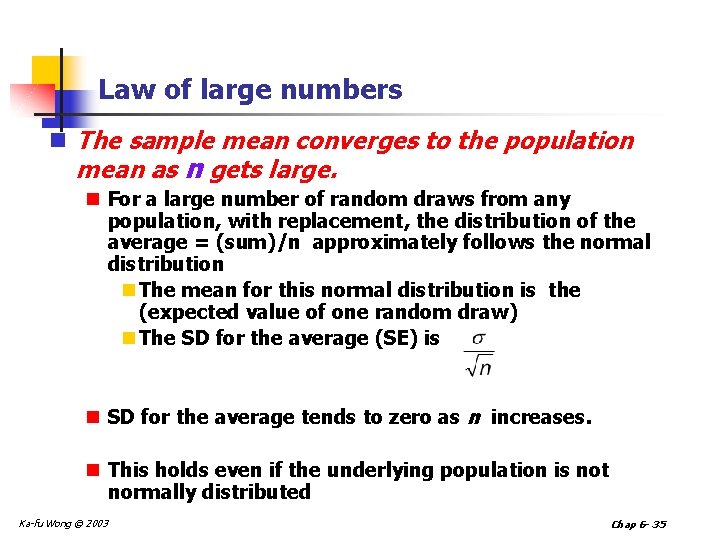
Law of large numbers n The sample mean converges to the population mean as n gets large. n For a large number of random draws from any population, with replacement, the distribution of the average = (sum)/n approximately follows the normal distribution n The mean for this normal distribution is the (expected value of one random draw) n The SD for the average (SE) is n SD for the average tends to zero as n increases. n This holds even if the underlying population is not normally distributed Ka-fu Wong © 2003 Chap 6 - 35

Point Estimates n Examples of point estimates are the sample mean, the sample standard deviation, the sample variance, the sample proportion. n A point estimate is one value ( a single point) that is used to estimate a population parameter. Ka-fu Wong © 2003 Chap 6 - 36

Independent identically distributed (iid) n “random draws from any population, with replacement” is also known as independent identically distributed. n Independent: the probability of drawing the current observation does not depend on what has been drawn previously. n Identically distributed: the probability of drawing the current observation is the same as what has been drawn previously and what will be drawn in the future. The CLT may still hold even when we do not have iid observations. Ka-fu Wong © 2003 Chap 6 - 37

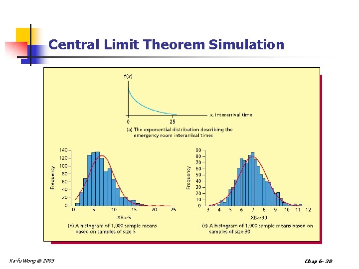
Central Limit Theorem Simulation Ka-fu Wong © 2003 Chap 6 - 38

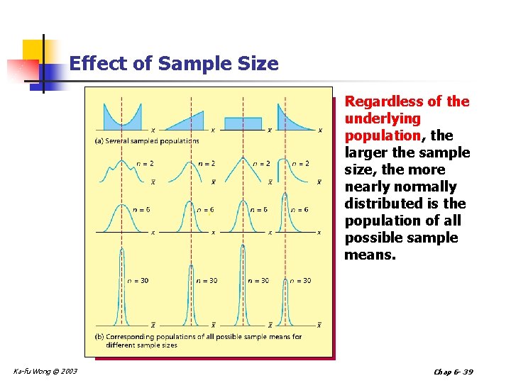
Effect of Sample Size Regardless of the underlying population, the larger the sample size, the more nearly normally distributed is the population of all possible sample means. Ka-fu Wong © 2003 Chap 6 - 39

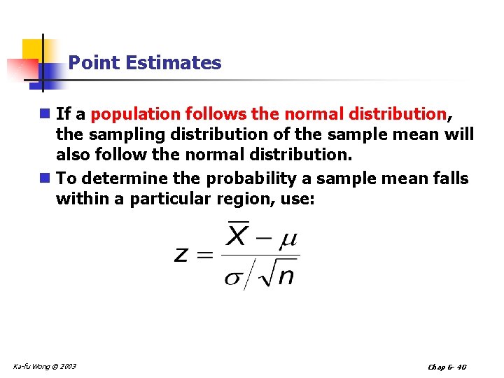
Point Estimates n If a population follows the normal distribution, the sampling distribution of the sample mean will also follow the normal distribution. n To determine the probability a sample mean falls within a particular region, use: Ka-fu Wong © 2003 Chap 6 - 40

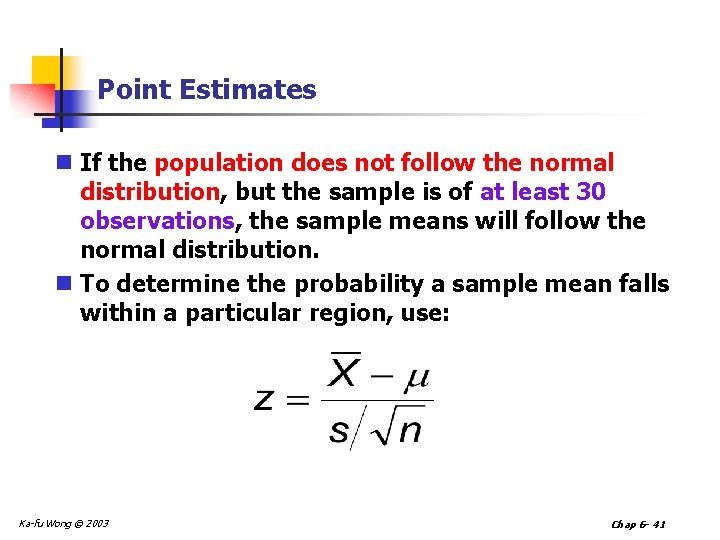
Point Estimates n If the population does not follow the normal distribution, but the sample is of at least 30 observations, the sample means will follow the normal distribution. n To determine the probability a sample mean falls within a particular region, use: Ka-fu Wong © 2003 Chap 6 - 41

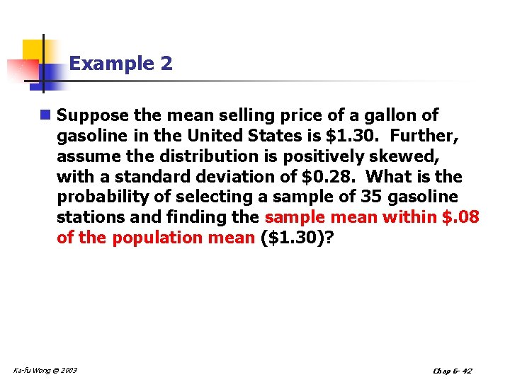
Example 2 n Suppose the mean selling price of a gallon of gasoline in the United States is $1. 30. Further, assume the distribution is positively skewed, with a standard deviation of $0. 28. What is the probability of selecting a sample of 35 gasoline stations and finding the sample mean within $. 08 of the population mean ($1. 30)? Ka-fu Wong © 2003 Chap 6 - 42

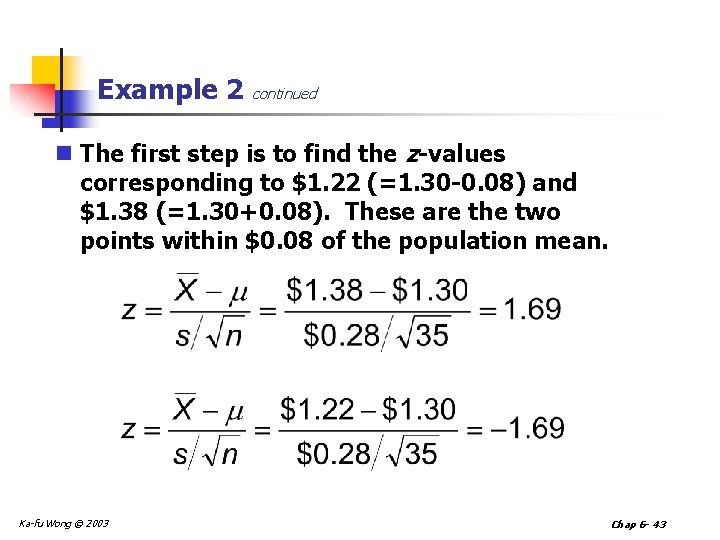
Example 2 continued n The first step is to find the z-values corresponding to $1. 22 (=1. 30 -0. 08) and $1. 38 (=1. 30+0. 08). These are the two points within $0. 08 of the population mean. Ka-fu Wong © 2003 Chap 6 - 43

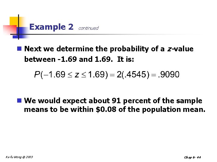
Example 2 continued n Next we determine the probability of a z-value between -1. 69 and 1. 69. It is: n We would expect about 91 percent of the sample means to be within $0. 08 of the population mean. Ka-fu Wong © 2003 Chap 6 - 44

Estimating the percentage of Earth covered by water n Experiments: n Paint a dot on your thumb. n Catch the globe and tell me whether the dot on your thumb land on water. n Estimate the percentage of Earth covered by water by the average of all trials. n Idea: If we draw many observations with replacement, the sample average will approach the population proportion. Code water as 1 and land as 0, the sample average will be an estimate of the proportion will be the percentage of Earth covered by water. Truth: Water covers 71% of the Earth's surface. e. g. , http: //pao. cnmoc. navy. mil/educate/neptune/trivia/earth. htm Ka-fu Wong © 2003 Chap 6 - 45

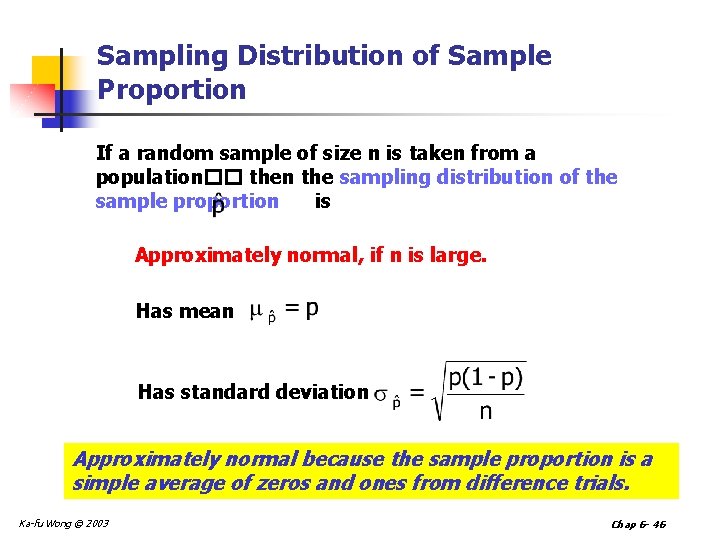
Sampling Distribution of Sample Proportion If a random sample of size n is taken from a population�� then the sampling distribution of the sample proportion is Approximately normal, if n is large. Has mean Has standard deviation Approximately normal because the sample proportion is a simple average of zeros and ones from difference trials. Ka-fu Wong © 2003 Chap 6 - 46

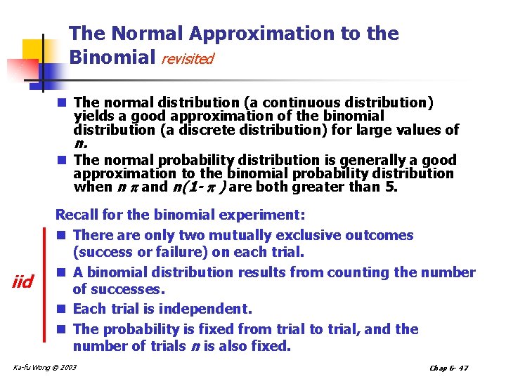
The Normal Approximation to the Binomial revisited n The normal distribution (a continuous distribution) yields a good approximation of the binomial distribution (a discrete distribution) for large values of n. n The normal probability distribution is generally a good approximation to the binomial probability distribution when n and n(1 - ) are both greater than 5. iid Recall for the binomial experiment: n There are only two mutually exclusive outcomes (success or failure) on each trial. n A binomial distribution results from counting the number of successes. n Each trial is independent. n The probability is fixed from trial to trial, and the number of trials n is also fixed. Ka-fu Wong © 2003 Chap 6 - 47

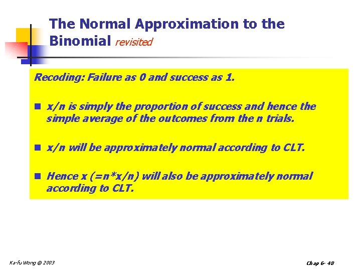
The Normal Approximation to the Binomial revisited Recoding: Failure as 0 and success as 1. n x/n is simply the proportion of success and hence the simple average of the outcomes from the n trials. n x/n will be approximately normal according to CLT. n Hence x (=n*x/n) will also be approximately normal according to CLT. Ka-fu Wong © 2003 Chap 6 - 48

Chapter six Sampling Methods and the Central Limit Theorem - END - Ka-fu Wong © 2003 Chap 6 - 49