Characterizing the Cyclical Component Kafu Wong University of

Characterizing the Cyclical Component Ka-fu Wong University of Hong Kong 1

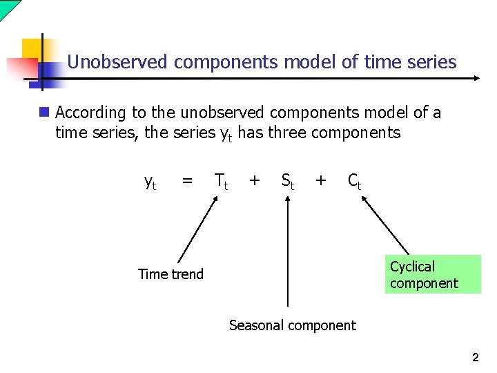
Unobserved components model of time series n According to the unobserved components model of a time series, the series yt has three components yt = Tt + St + Ct Cyclical component Time trend Seasonal component 2

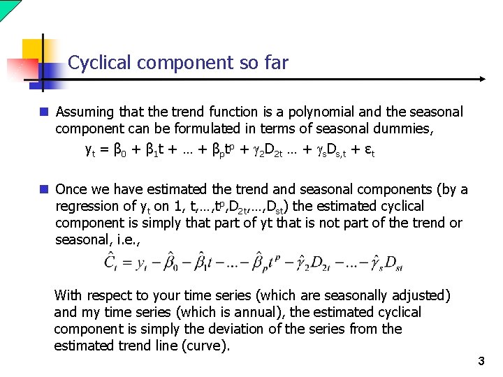
Cyclical component so far n Assuming that the trend function is a polynomial and the seasonal component can be formulated in terms of seasonal dummies, yt = β 0 + β 1 t + … + βptp + g 2 D 2 t … + gs. Ds, t + εt n Once we have estimated the trend and seasonal components (by a regression of yt on 1, t, …, tp, D 2 t, …, Dst) the estimated cyclical component is simply that part of yt that is not part of the trend or seasonal, i. e. , With respect to your time series (which are seasonally adjusted) and my time series (which is annual), the estimated cyclical component is simply the deviation of the series from the estimated trend line (curve). 3

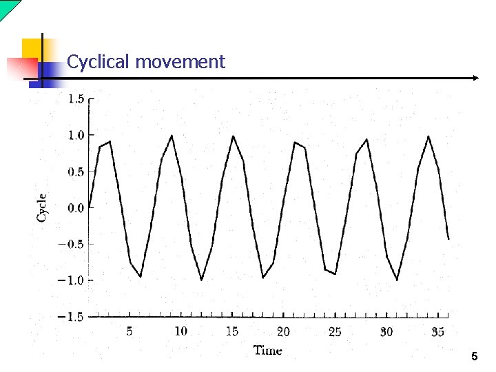
Possible to predict the cyclical components n So far we have been assuming that the cyclical component is made up of the outcomes of drawings of i. i. d. random variables, which is simple but not very plausible. n Generally, there is some predictability in the cyclical component. 4

Cyclical movement 5

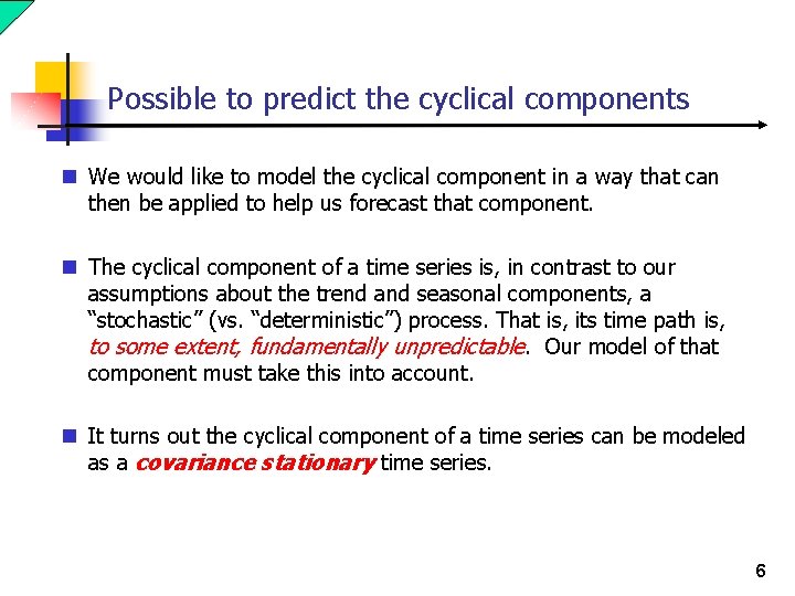
Possible to predict the cyclical components n We would like to model the cyclical component in a way that can then be applied to help us forecast that component. n The cyclical component of a time series is, in contrast to our assumptions about the trend and seasonal components, a “stochastic” (vs. “deterministic”) process. That is, its time path is, to some extent, fundamentally unpredictable. Our model of that component must take this into account. n It turns out the cyclical component of a time series can be modeled as a covariance stationary time series. 6

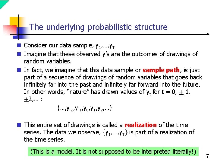
The underlying probabilistic structure n Consider our data sample, y 1, …, y. T n Imagine that these observed y’s are the outcomes of drawings of random variables. n In fact, we imagine that this data sample or sample path, is just part of a sequence of drawings of random variables that goes back infinitely far into the past and infinitely far forward into the future. In other words, “nature” has drawn values of yt for t = 0, + 1, +2, … : {…, y-2, y-1, y 0, y 1, y 2, …} n This entire set of drawings is called a realization of the time series. The data we observe, {y 1, …, y. T} is part of a realization of the time series. (This is a model. It is not supposed to be interpreted literally!) 7

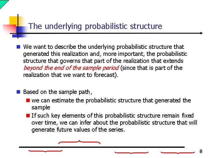
The underlying probabilistic structure n We want to describe the underlying probabilistic structure that generated this realization and, more important, the probabilistic structure that governs that part of the realization that extends beyond the end of the sample period (since that is part of the realization that we want to forecast). n Based on the sample path, n we can estimate the probabilistic structure that generated the sample n If such key elements of this probabilistic structure remain fixed over time, we can infer about the probabilistic structure that will generate future values of the series. 8

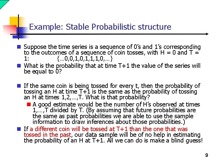
Example: Stable Probabilistic structure n Suppose the time series is a sequence of 0’s and 1’s corresponding to the outcomes of a sequence of coin tosses, with H = 0 and T = 1: {… 0, 0, 1, 1, 1, 0, …} n What is the probability that at time T+1 the value of the series will be equal to 0? n If the same coin is being tossed for every t, then the probability of tossing an H at time T+1 is the same as the probability of tossing an H at times 1, 2, …, T. What is that probability? n A good estimate would be the number of H’s observed at times 1, …, T divided by T. (By assuming that future probabilities are the same as past probabilities we are able to use the sample information to draw inferences about those probabilities. ) n If a different coin will be tossed at T+1 than the one that was tossed in the past, our data sample will be of no help in estimating the probability of an H at T+1. All we can do is make a blind guess! 9

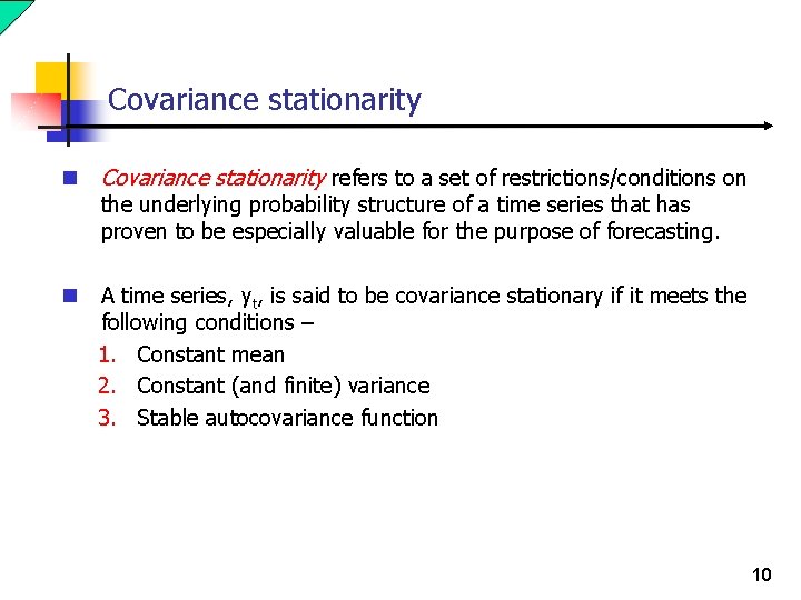
Covariance stationarity n Covariance stationarity refers to a set of restrictions/conditions on n A time series, yt, is said to be covariance stationary if it meets the following conditions – 1. Constant mean 2. Constant (and finite) variance 3. Stable autocovariance function the underlying probability structure of a time series that has proven to be especially valuable for the purpose of forecasting. 10

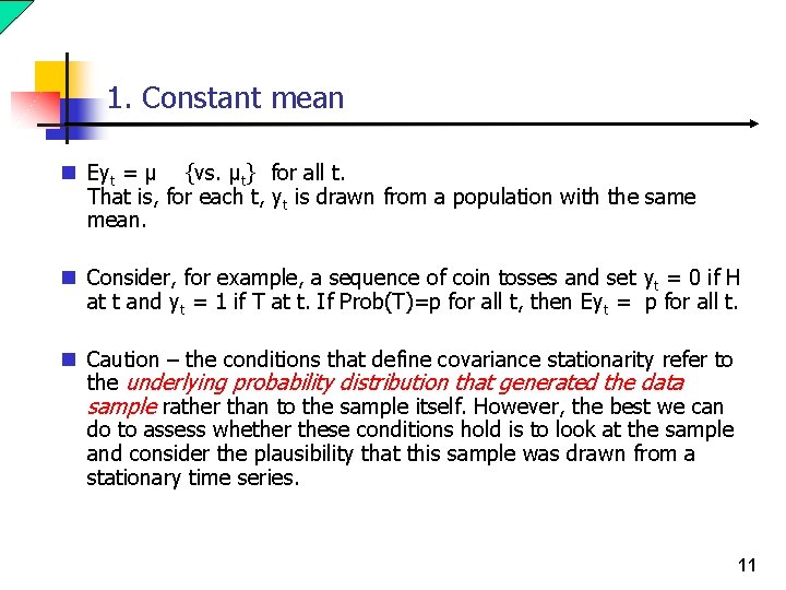
1. Constant mean n Eyt = μ {vs. μt} for all t. That is, for each t, yt is drawn from a population with the same mean. n Consider, for example, a sequence of coin tosses and set yt = 0 if H at t and yt = 1 if T at t. If Prob(T)=p for all t, then Eyt = p for all t. n Caution – the conditions that define covariance stationarity refer to the underlying probability distribution that generated the data sample rather than to the sample itself. However, the best we can do to assess whether these conditions hold is to look at the sample and consider the plausibility that this sample was drawn from a stationary time series. 11

2. Constant Variance n Var(yt) = E[(yt- μ)2] = σ2 {vs. σt 2} for all t. n That is, the dispersion of the value of yt around its mean is constant over time. n A sample in which the dispersion of the data around the sample mean seems to be increasing or decreasing over time is not likely to have been drawn from a time series with a constant variance. n Consider, for example, a sequence of coin tosses and set yt = 0 if H at t and yt = 1 if T at t. If Prob(T)=p for all t, then, for all t n Eyt = p and n Var(yt) = E[(yt – p)2] = p(1 -p)2+(1 -p)p 2 = p(1 -p). 12

Digression on covariance and correlation n Recall that n Cov(X, Y) = E[(X-EX)(Y-EY)], and n Corr(X, Y) = Cov(X, Y)/[Var(X)Var(Y)]1/2 measure the relationship between the random variables X and Y. n A positive covariance means that when X > EX, Y will tend to be greater than EY (and vice versa). n A negative covariance means that when X > EX, Y will tend to be less than EY (and vice versa). 13

Digression on covariance and correlation n Cov(X, Y) = E[(X-EX)(Y-EY)], and n Corr(X, Y) = Cov(X, Y)/[Var(X)Var(Y)]1/2 n The correlation between X and Y will have the same sign as the covariance but its value will lie between -1 and 1. The stronger the relationship between X and Y, the closer their correlation will be to 1 (or, in the case of negative correlation, -1). n If the correlation is 1, X and Y are perfectly positively correlated. If the correlation is -1, X and Y are perfectly negatively correlated. X and Y are uncorrelated if the correlation is 0. n Remark: Independent random variables are uncorrelated. Uncorrelated random variables are not necessarily independent. 14

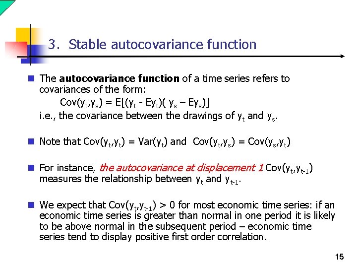
3. Stable autocovariance function n The autocovariance function of a time series refers to covariances of the form: Cov(yt, ys) = E[(yt - Eyt)( ys – Eys)] i. e. , the covariance between the drawings of yt and ys. n Note that Cov(yt, yt) = Var(yt) and Cov(yt, ys) = Cov(ys, yt) n For instance, the autocovariance at displacement 1 Cov(yt, yt-1) measures the relationship between yt and yt-1. n We expect that Cov(yt, yt-1) > 0 for most economic time series: if an economic time series is greater than normal in one period it is likely to be above normal in the subsequent period – economic time series tend to display positive first order correlation. 15

3. Stable autocovariance function n In the coin toss example (yt = 0 if H, yt = 1 if T), what is Cov(yt, yt-1)? 16

3. Stable autocovariance function n Suppose that Cov(yt, yt-1) = g(1) for all t where g(1) is some constant. n That is, the autocovariance at displacement 1 is the same for all t: …Cov(y 2, y 1)=Cov(y 3, y 2)=…=Cov(y. T, y. T-1)=… n In this special case, we might also say that the autocovariance at displacement 1 is stable over time. 17

3. Stable autocovariance function n The third condition for covariance stationarity is that the autocovariance function is stable at all displacements. That is – Cov(yt, yt-t) = g(t) for all integers t and t n The covariance between yt and ys depends on t and s only through t-s (how far apart they are in time) not on t and s themselves (where they are in time). Cov(y 1, y 3)=Cov(y 2, y 4) =…=Cov(y. T-2, y. T) = g(2) and so on. n Stationarity means if we break the entire time series up into different segments, the general behavior of the series looks roughly the same for each segment. 18

3. Stable autocovariance function n Remark #1: Note that stability of the autocovariance function (condition 3) actually implies a constant variance (condition 2) {set t = 0. } n Remark #2: g(t) = g (-t) since g(t) = Cov(yt, yt-t) = Cov(yt-t, yt) = g (-t) n Remark #3: If yt is an i. i. d. sequence of random variables then it is a covariance stationary time series. {The “identical distribution” means that the mean and variance are the same for all t. The independence assumption means that g(t) = 0 for all nonzero t, which implies a stable autocovariance function. } 19

3. Stable autocovariance function n The conditions for covariance stationary are the main conditions we will need regarding the stability of the probability structure generating the time series in order to be able to use the past to help us predict the future. n Remark: It is important to note that these conditions n do not imply that the y’s are identically distributed (or, independent). n do not place restrictions on third, fourth, and higher order moments (skewness, kurtosis, …). [Covariance stationarity only restricts the first two moments and so it also referred to as “second-order stationarity. ”] 20

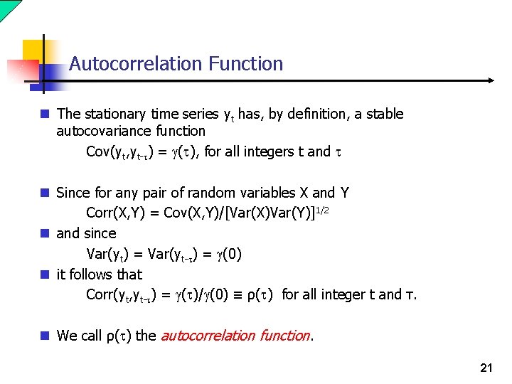
Autocorrelation Function n The stationary time series yt has, by definition, a stable autocovariance function Cov(yt, yt-t) = g(t), for all integers t and t n Since for any pair of random variables X and Y Corr(X, Y) = Cov(X, Y)/[Var(X)Var(Y)]1/2 n and since Var(yt) = Var(yt-t) = g(0) n it follows that Corr(yt, yt-t) = g(t)/g(0) ≡ ρ(t) for all integer t and τ. n We call ρ(t) the autocorrelation function. 21

Autocorrelation Function n The autocorrelation and autocovariance functions provide the same information about the relationship of the y’s across time, but in different ways. It turns out that the autocorrelation function is more useful in applications of this theory, such as ours. n The way we will use the autocorrelation function – n Each member of the class of candidate models will have a unique autocorrelation function that will identify it, much like a fingerprint or DNA uniquely identifies an individual in a population of humans. n We will estimate the autocorrelation function of the series (i. e. , get a partial fingerprint) and use that to help us select the appropriate model. 22

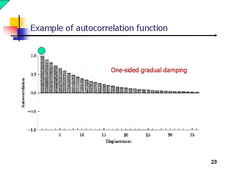
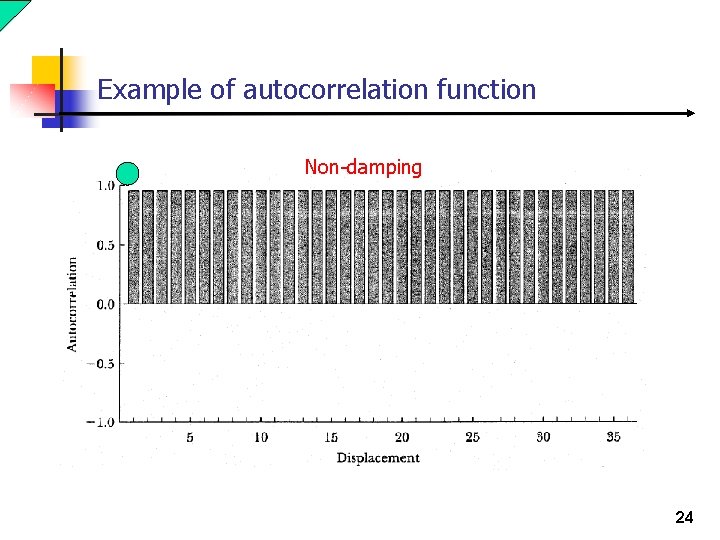
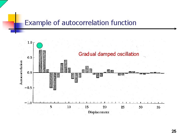
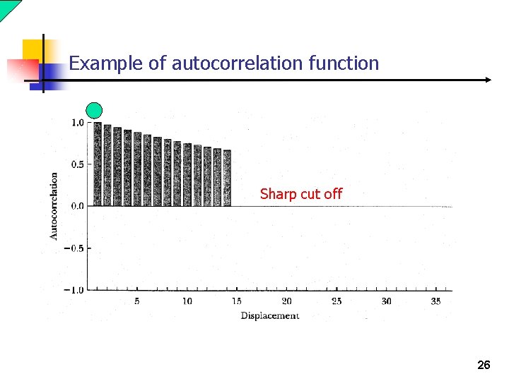
Example of autocorrelation function One-sided gradual damping 23

Example of autocorrelation function Non-damping 24

Example of autocorrelation function Gradual damped oscillation 25

Example of autocorrelation function Sharp cut off 26

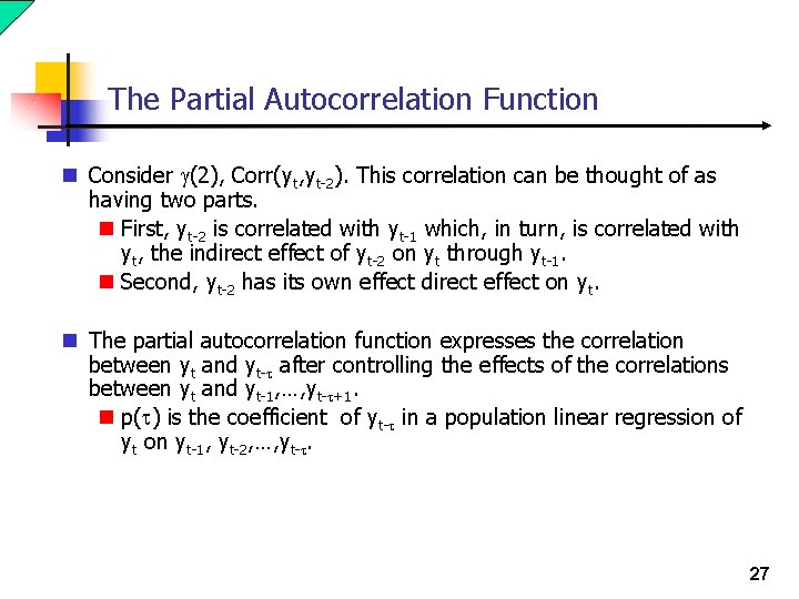
The Partial Autocorrelation Function n Consider g(2), Corr(yt, yt-2). This correlation can be thought of as having two parts. n First, yt-2 is correlated with yt-1 which, in turn, is correlated with yt, the indirect effect of yt-2 on yt through yt-1. n Second, yt-2 has its own effect direct effect on yt. n The partial autocorrelation function expresses the correlation between yt and yt-t after controlling the effects of the correlations between yt and yt-1, …, yt-t+1. n p(t) is the coefficient of yt-t in a population linear regression of yt on yt-1, yt-2, …, yt-t. 27

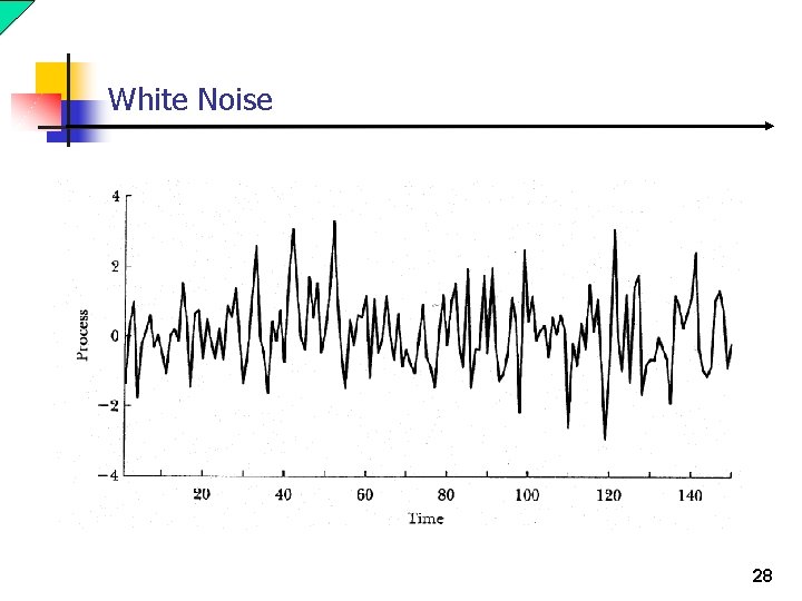
White Noise 28

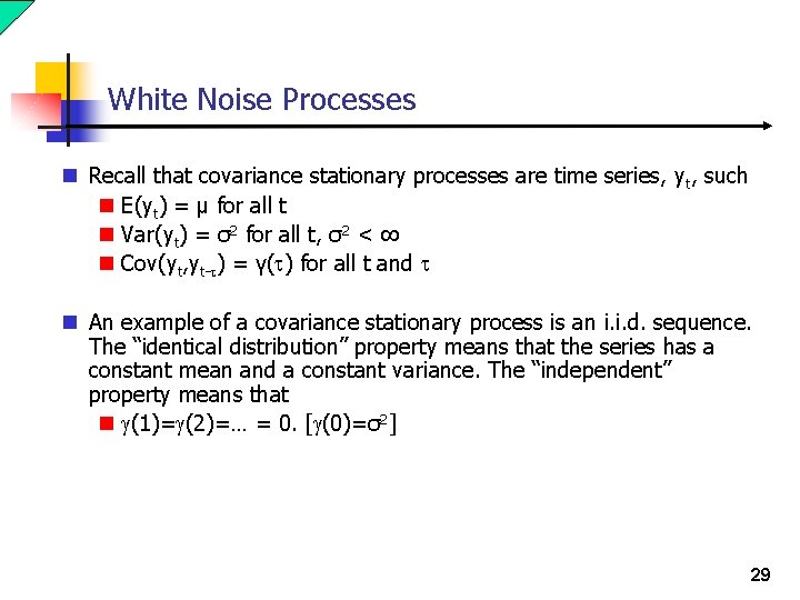
White Noise Processes n Recall that covariance stationary processes are time series, yt, such n E(yt) = μ for all t n Var(yt) = σ2 for all t, σ2 < ∞ n Cov(yt, yt-t) = γ(t) for all t and t n An example of a covariance stationary process is an i. i. d. sequence. The “identical distribution” property means that the series has a constant mean and a constant variance. The “independent” property means that n g(1)=g(2)=… = 0. [g(0)=σ2] 29

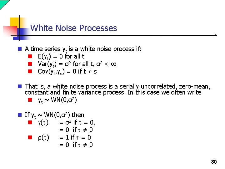
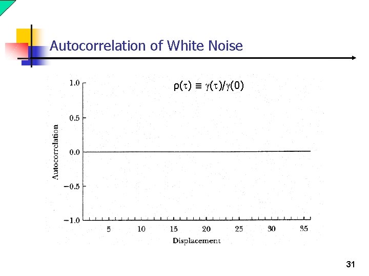
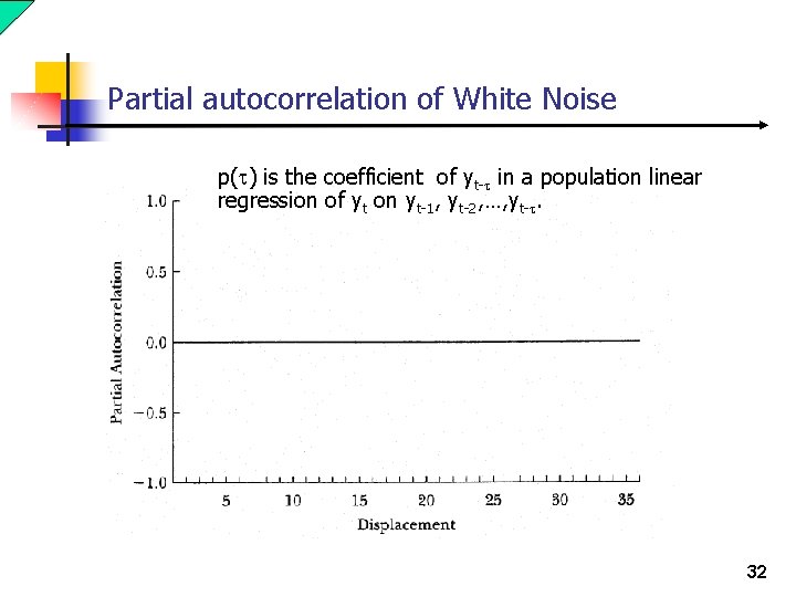
White Noise Processes n A time series yt is a white noise process if: n E(yt) = 0 for all t n Var(yt) = σ2 for all t, σ2 < ∞ n Cov(yt, ys) = 0 if t ≠ s n That is, a white noise process is a serially uncorrelated, zero-mean, constant and finite variance process. In this case we often write n yt ~ WN(0, σ2) n If yt ~ WN(0, σ2) then n g(t) = σ2 if t = 0, = 0 if t ≠ 0 n ρ(t) = 1 if t = 0 if t ≠ 0 30

Autocorrelation of White Noise ρ(t) ≡ g(t)/g(0) 31

Partial autocorrelation of White Noise p(t) is the coefficient of yt-t in a population linear regression of yt on yt-1, yt-2, …, yt-t. 32

White Noise Processes n Remark #1: Technically, an i. i. d. process (with a finite variance) is a white noise process but a white noise process is not necessarily an i. i. d. process (since the y’s are not necessarily identically distributed or independent). However, for most of our purposes we will use these two interchangeably. n Remark #2: In regression models we often assume that the regression errors are zero-mean, homoskedastic, and serially uncorrelated random variables, i. e. , they are white noise errors. 33

White Noise Processes n In our study of the trend and seasonal components, we assumed that the cyclical component of the series was a white noise process and, therefore, was unpredictable. That was a convenient assumption at the time. n We now want to allow the cyclical component to be a serially correlated process, since our graphs of the deviations of our seasonally adjusted series from their estimated trends indicate that these deviations do not behave like white noise. n However, the white noise process will still be very important to us: It forms the basic building block for the construction of more complicated time series. 34

Estimating the Autocorrelation Function n Soon we will specify the class of models that we will use for covariance stationary processes. These models (ARMA and ARIMA models) are built up from the white noise process. We will use the estimated autocorrelation and partial autocorrelation functions of the series to help us select the particular model that we will estimate to help us forecast the series. n How to estimate the autocorrelation function? n The principle we use is referred to in your textbook as the analog principle. The analog principle, which turns out to have a sound basis in statistical theory, is to estimate population moments by the analogous sample moment, i. e. , replace expected values with analogous sample averages. 35

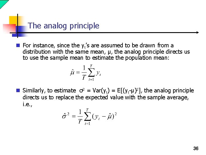
The analog principle n For instance, since the yt’s are assumed to be drawn from a distribution with the same mean, μ, the analog principle directs us to use the sample mean to estimate the population mean: n Similarly, to estimate σ2 = Var(yt) = E[(yt-μ)2], the analog principle directs us to replace the expected value with the sample average, i. e. , 36

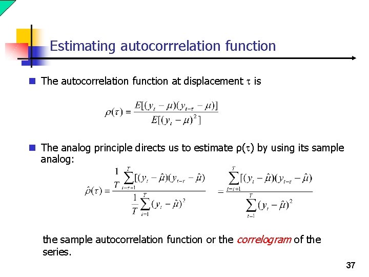
Estimating autocorrrelation function n The autocorrelation function at displacement t is n The analog principle directs us to estimate ρ(t) by using its sample analog: the sample autocorrelation function or the correlogram of the series. 37

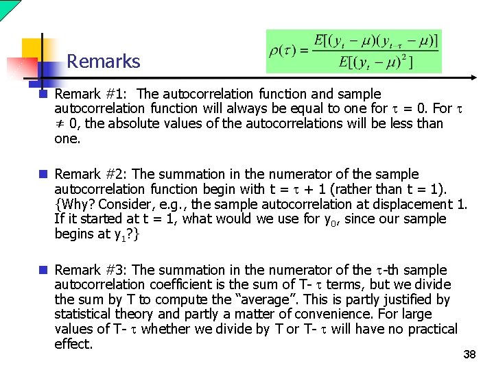
Remarks n Remark #1: The autocorrelation function and sample autocorrelation function will always be equal to one for t = 0. For t ≠ 0, the absolute values of the autocorrelations will be less than one. n Remark #2: The summation in the numerator of the sample autocorrelation function begin with t = t + 1 (rather than t = 1). {Why? Consider, e. g. , the sample autocorrelation at displacement 1. If it started at t = 1, what would we use for y 0, since our sample begins at y 1? } n Remark #3: The summation in the numerator of the t-th sample autocorrelation coefficient is the sum of T- t terms, but we divide the sum by T to compute the “average”. This is partly justified by statistical theory and partly a matter of convenience. For large values of T- t whether we divide by T or T- t will have no practical effect. 38

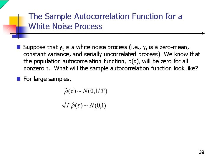
The Sample Autocorrelation Function for a White Noise Process n Suppose that yt is a white noise process (i. e. , yt is a zero-mean, constant variance, and serially uncorrelated process). We know that the population autocorrelation function, ρ(t), will be zero for all nonzero t. What will the sample autocorrelation function look like? n For large samples, 39

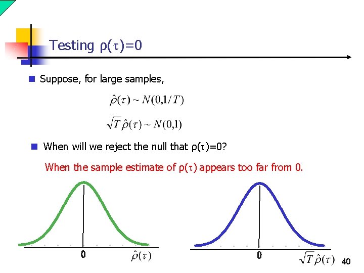
Testing ρ(t)=0 n Suppose, for large samples, n When will we reject the null that ρ(t)=0? When the sample estimate of ρ(t) appears too far from 0. 0 0 40

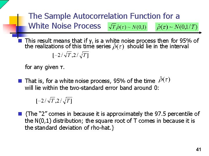
The Sample Autocorrelation Function for a White Noise Process n This result means that if yt is a white noise process then for 95% of the realizations of this time series should lie in the interval for any given τ. n That is, for a white noise process, 95% of the time will lie within the two-standard error band around 0: n {The “ 2” comes in because it is approximately the 97. 5 percentile of the N(0, 1) distribution; the square root of T comes in because it is the standard deviation of rho-hat. } 41

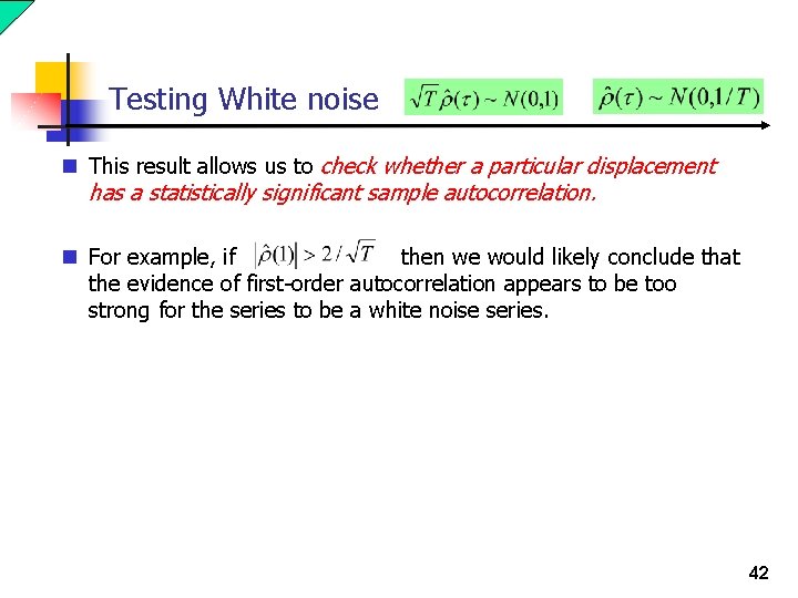
Testing White noise n This result allows us to check whether a particular displacement has a statistically significant sample autocorrelation. n For example, if then we would likely conclude that the evidence of first-order autocorrelation appears to be too strong for the series to be a white noise series. 42

Testing white noise n However, it is not reasonable to say that you will reject the white noise hypothesis if any of the rho-hats falls outside of the twostandard error band around zero. n Why not? Because even if the series is a white noise series, we expect some of the sample autocorrelations to fall outside that band – the band was constructed so that most of the sample autocorrelations would typically fall within the band if the time series is a realization of a white noise process. n A better way to conduct a general test of the null hypothesis of a zero autocorrelation function (i. e. , white noise) against the alternative of a nonzero autocorrelation function is to conduct a Qtest. 43

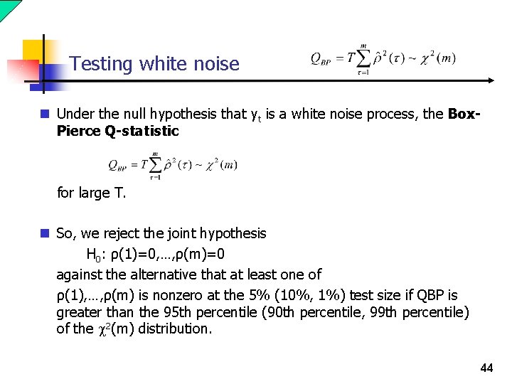
Testing white noise n Under the null hypothesis that yt is a white noise process, the Box. Pierce Q-statistic for large T. n So, we reject the joint hypothesis H 0: ρ(1)=0, …, ρ(m)=0 against the alternative that at least one of ρ(1), …, ρ(m) is nonzero at the 5% (10%, 1%) test size if QBP is greater than the 95 th percentile (90 th percentile, 99 th percentile) of the c 2(m) distribution. 44

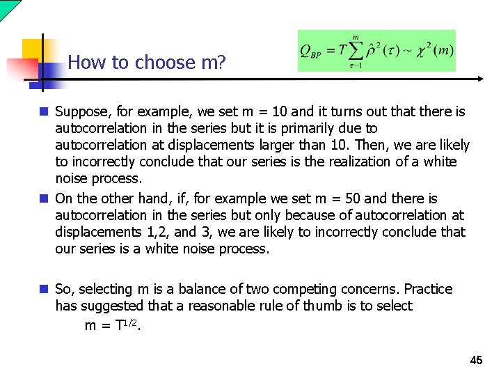
How to choose m? n Suppose, for example, we set m = 10 and it turns out that there is autocorrelation in the series but it is primarily due to autocorrelation at displacements larger than 10. Then, we are likely to incorrectly conclude that our series is the realization of a white noise process. n On the other hand, if, for example we set m = 50 and there is autocorrelation in the series but only because of autocorrelation at displacements 1, 2, and 3, we are likely to incorrectly conclude that our series is a white noise process. n So, selecting m is a balance of two competing concerns. Practice has suggested that a reasonable rule of thumb is to select m = T 1/2. 45

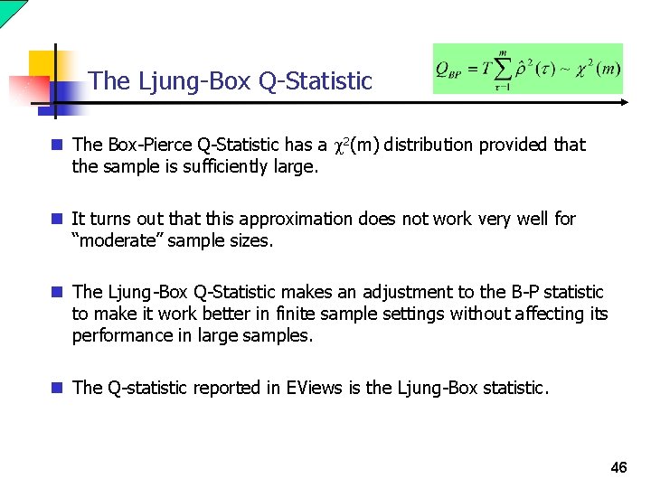
The Ljung-Box Q-Statistic n The Box-Pierce Q-Statistic has a c 2(m) distribution provided that the sample is sufficiently large. n It turns out that this approximation does not work very well for “moderate” sample sizes. n The Ljung-Box Q-Statistic makes an adjustment to the B-P statistic to make it work better in finite sample settings without affecting its performance in large samples. n The Q-statistic reported in EViews is the Ljung-Box statistic. 46

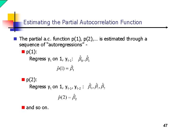
Estimating the Partial Autocorrelation Function n The partial a. c. function p(1), p(2), … is estimated through a sequence of “autoregressions” n p(1): Regress yt on 1, yt-1: n p(2): Regress yt on 1, yt-2 : n and so on. 47

End 48