Volatility Smiles What is a Volatility Smile n

Volatility Smiles

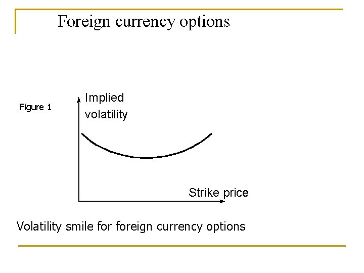
What is a Volatility Smile? n It is the relationship between implied volatility and strike price for options with a certain maturity

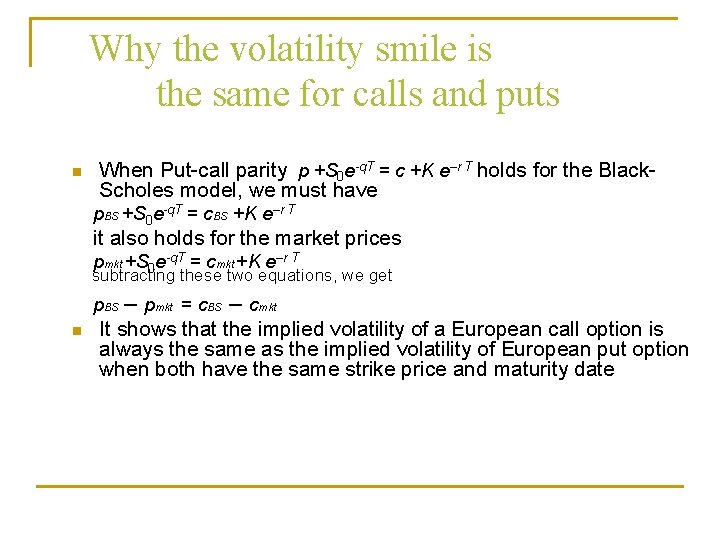
Why the volatility smile is the same for calls and puts n When Put-call parity p +S 0 e-q. T = c +K e–r T holds for the Black. Scholes model, we must have p. BS +S 0 e-q. T = c. BS +K e–r T it also holds for the market prices pmkt +S 0 e-q. T = cmkt +K e–r T subtracting these two equations, we get p. BS － pmkt = c. BS － cmkt n It shows that the implied volatility of a European call option is always the same as the implied volatility of European put option when both have the same strike price and maturity date

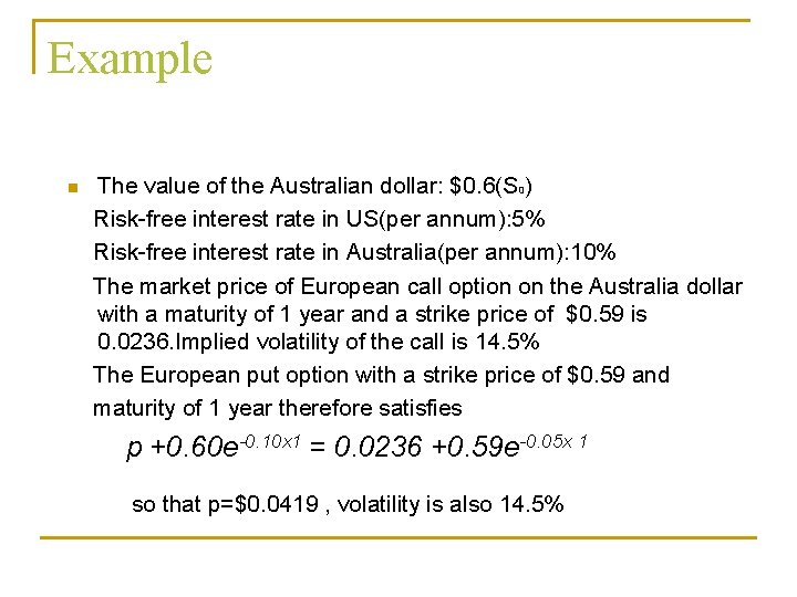
Example n The value of the Australian dollar: $0. 6(S 0) Risk-free interest rate in US(per annum): 5% Risk-free interest rate in Australia(per annum): 10% The market price of European call option on the Australia dollar with a maturity of 1 year and a strike price of $0. 59 is 0. 0236. Implied volatility of the call is 14. 5% The European put option with a strike price of $0. 59 and maturity of 1 year therefore satisfies p +0. 60 e-0. 10 x 1 = 0. 0236 +0. 59 e-0. 05 x 1 so that p=$0. 0419 , volatility is also 14. 5%

Foreign currency options Figure 1 Implied volatility Strike price Volatility smile foreign currency options

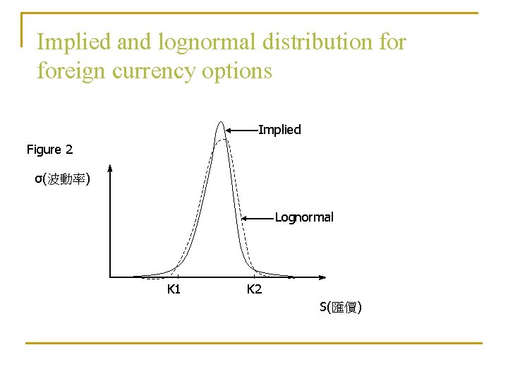
Implied and lognormal distribution foreign currency options Implied Figure 2 σ(波動率) Lognormal K 1 K 2 S(匯價)

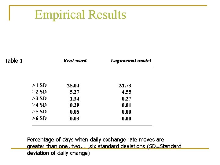
Empirical Results Table 1 Real word >1 SD >2 SD >3 SD >4 SD >5 SD >6 SD 25. 04 5. 27 1. 34 0. 29 0. 08 0. 03 Lognormal model 31. 73 4. 55 0. 27 0. 01 0. 00 Percentage of days when daily exchange rate moves are greater than one, two, … , six standard deviations (SD=Standard deviation of daily change)

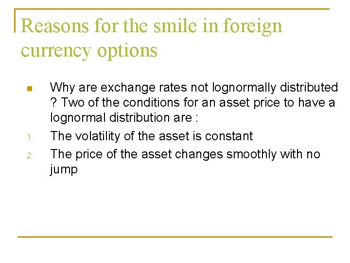
Reasons for the smile in foreign currency options n 1. 2. Why are exchange rates not lognormally distributed ? Two of the conditions for an asset price to have a lognormal distribution are : The volatility of the asset is constant The price of the asset changes smoothly with no jump

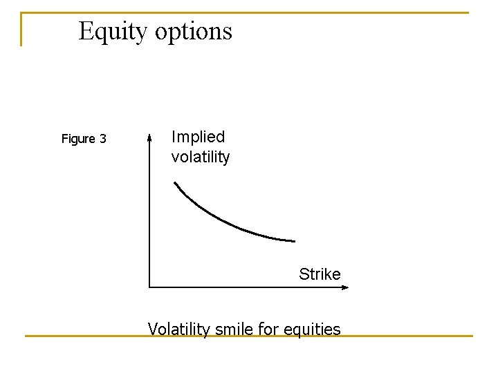
Equity options Figure 3 Implied volatility Strike Volatility smile for equities

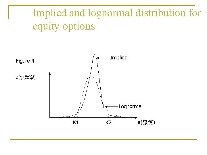
Implied and lognormal distribution for equity options Implied Figure 4 σ(波動率) Lognormal K 1 K 2 s(股價)

The reason for the smile in equity options n n One possible explanation for the smile in equity options concerns leverage Another explanation is “crashophobia”

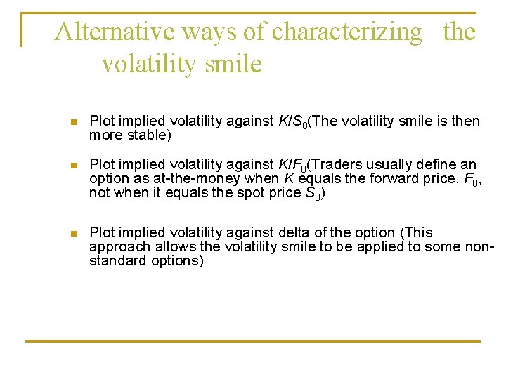
Alternative ways of characterizing the volatility smile n Plot implied volatility against K/S 0(The volatility smile is then more stable) n Plot implied volatility against K/F 0(Traders usually define an option as at-the-money when K equals the forward price, F 0, not when it equals the spot price S 0) n Plot implied volatility against delta of the option (This approach allows the volatility smile to be applied to some nonstandard options)

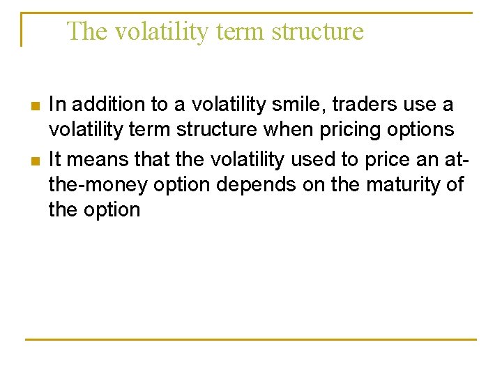
The volatility term structure n n In addition to a volatility smile, traders use a volatility term structure when pricing options It means that the volatility used to price an atthe-money option depends on the maturity of the option

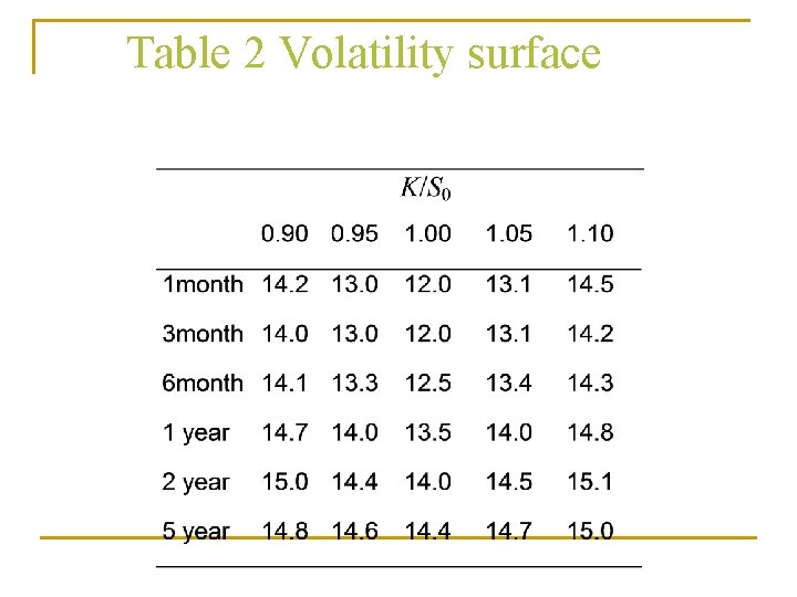
The volatility surfaces n Volatility surfaces combine volatility smiles with the volatility term structure to tabulate the volatilities appropriate for pricing an option with any strike price and any maturity

Table 2 Volatility surface

The volatility surfaces n The shape of the volatility smile depends on the option maturity. As illustrated in Table 2, the smile tends to become less pronounced as the option maturity increases

Greek letters n n The volatility smile complicate the calculation of Greek letters Assume that the relationship between the implied volatility and K/S for an option with a certain time to maturity remains the same

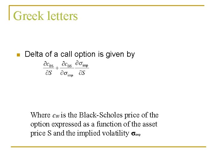
Greek letters n Delta of a call option is given by Where c. BS is the Black-Scholes price of the option expressed as a function of the asset price S and the implied volatility σimp

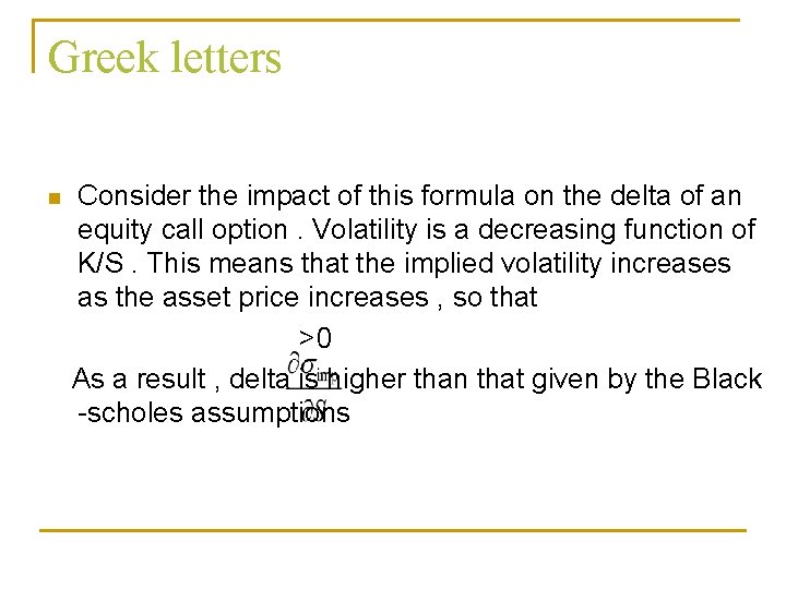
Greek letters n Consider the impact of this formula on the delta of an equity call option. Volatility is a decreasing function of K/S. This means that the implied volatility increases as the asset price increases , so that >0 As a result , delta is higher than that given by the Black -scholes assumptions

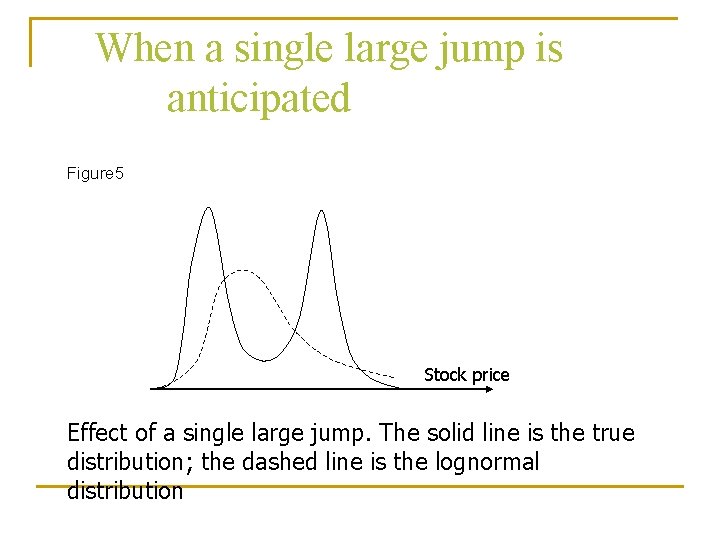
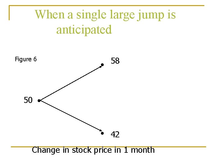
When a single large jump is anticipated n Suppose that a stock price is currently $50 and an important news announcement due in a few days is expected either to increase the stock price by $8 or to reduce it by $8. The probability distribution the stock price in 1 month might consist of a mixture of two lognormal distributions, the first corresponding to favorable news, the second to unfavorable news. The situation is illustrated in Figure 5.

When a single large jump is anticipated Figure 5 Stock price Effect of a single large jump. The solid line is the true distribution; the dashed line is the lognormal distribution

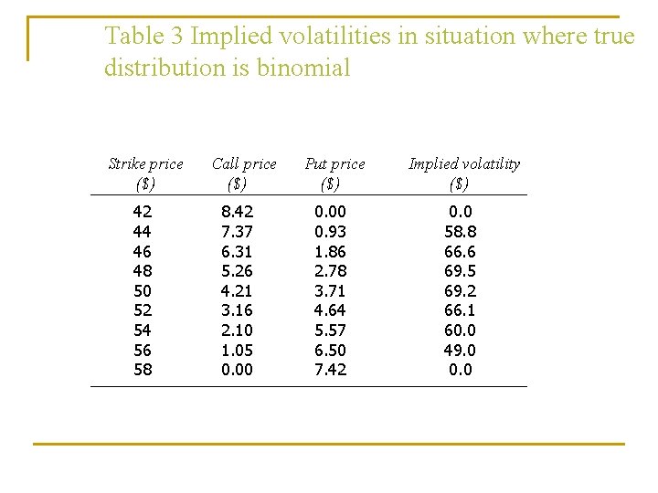
When a single large jump is anticipated n Suppose further that the risk-free rate is 12% per annum. The situation is illustrated in Figure 6. Options can be valued using the binomial model from Chapter 11. In this case u=1. 16, d=0. 84, a=1. 0101, and p=0. 5314 The results from valuing a range of different options are shown in Table 3

When a single large jump is anticipated Figure 6 50 ● 58 ● 42 ● Change in stock price in 1 month

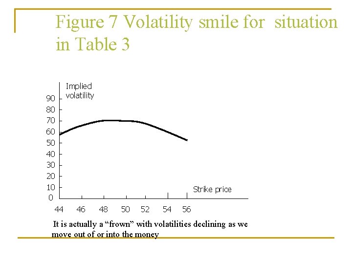
Table 3 Implied volatilities in situation where true distribution is binomial Strike price ($) 42 44 46 48 50 52 54 56 58 Call price ($) 8. 42 7. 37 6. 31 5. 26 4. 21 3. 16 2. 10 1. 05 0. 00 Put price ($) Implied volatility ($) 0. 00 0. 93 1. 86 2. 78 3. 71 4. 64 5. 57 6. 50 7. 42 0. 0 58. 8 66. 6 69. 5 69. 2 66. 1 60. 0 49. 0 0. 0

Figure 7 Volatility smile for situation in Table 3 90 80 70 60 50 40 30 20 10 0 44 Implied volatility Strike price 46 48 50 52 54 56 It is actually a “frown” with volatilities declining as we move out of or into the money