VIII Macroeconomic changes in the earlymodern European economy

VIII. Macro-economic changes in the early-modern European economy C. Price Movements during the Price Revolution and ‘General Crisis’ eras revised 26 January 2012

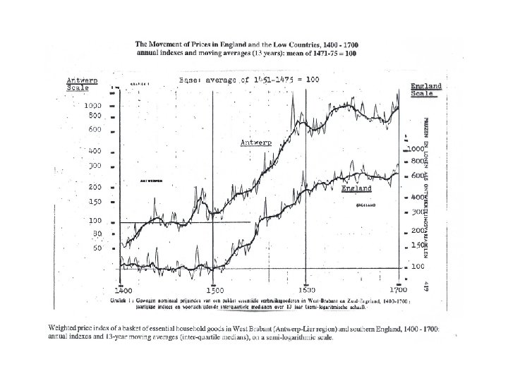
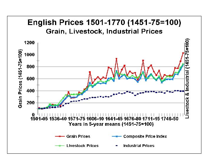
Price Revolution: Introduction • (1) Historical significance: • - while inflationary & deflationary cycles are a constant theme of European economic history, from the 12 th century to present day, the Price Revolution era is unique: • - longest sustained period of inflation ever recorded, • - importance: changes in both the price level (CPI) and changes in relative prices often had very major impacts on economic changes and economic growth: • especially in the agricultural and industrial sectors: in early modern Europe (from ca. 1500 to 1750: eve of Industrial Revolution) • I will later contend that most technological innovations were in response to changes in relative factor costs

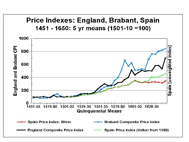
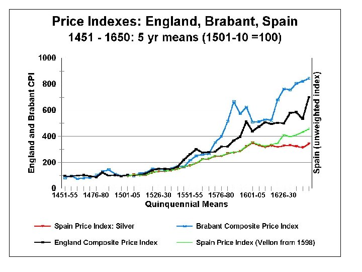
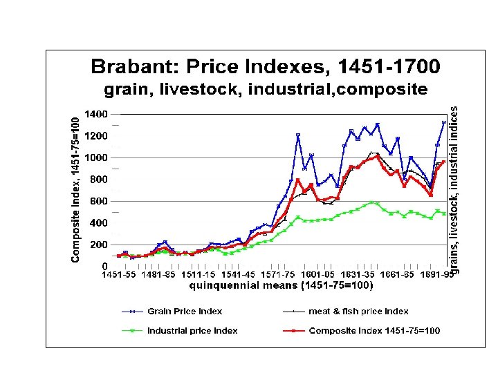
Price Revolution in England

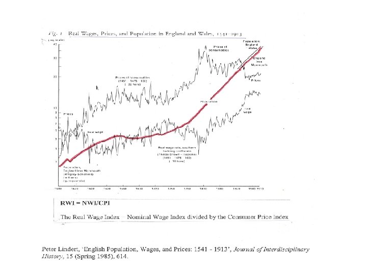
Price Revolution: Introduction (2) • (2) Debate about causes of the Price Revolution • (a) The Real School: that demographic factors (population growth) provided the primary (or even sole) cause – as suggested in the Lindert graph • - in my view, this thesis is badly mistaken: • - confuses micro-economics with macroeconomics; and • - confuses changes in relative prices with changes in the price level (CPI)

Price Revolution: Introduction (3) • (2) Debate about causes of the Price Revolution • (b) The Monetary School: that inflation & deflation are essentially monetary phenomena • - What is the more important: changes in stocks (money supplies) or in flows (income velocity)? • - not, however, purely a monetary phenom: • - demographic factors probably played some role in income-velocity changes: to be demonstrated later • - changes in aggregate output (NNI) = ‘y’: endogenous or exogenous to population growth? • (c) how and why are modern inflations different: in nature & form, from World War I?

Quantity Theories of Money 1 • (1) Fisher Identity: Equation of Exchange: M. V. = P. T - based on the transactions velocity of money - fault: impossibility of measuring transactions • (2) Friedman Version: M. V = P. y - based on the income velocity of money - y = Net National Income - deflated by CPI • - in both: distinguish between monetary stocks (M) and monetary flows (V)

Quantity Theories of Money 2 • (3) Cambridge Cash Balances (modernized) • - M = k. P. y • - in which ‘k’ measures that proportion of NNI (P. y) that the public chooses to hold in active cash balances (with no investment yield): • so that M = the quantity of money necessary to satisfy that equation • - Cambridge ‘k’: also seen as the propensity to hoard (without earning investment income)

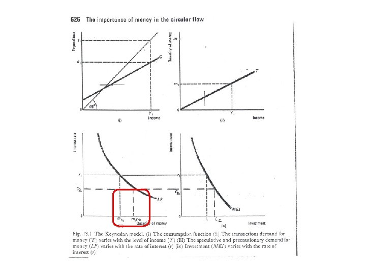
Quantity Theories of Money - 3 • (4) Keynes: Liquidity Preference: • the component factors explaining ‘k’: to hold active cash balances (instead of spending or investing) • - transactions motive • - precautionary motive (for a ‘rainy day’) • - investment + speculative motive • opportunity cost of ‘k’: forgoing income earned from investing those same funds • - Cambridge ‘k’ = reciprocal of Friedman ‘V’: i. e, the Income Velocity of Money • k = 1/V; V = 1/k

Quantity Theories of Money - 4 • (5) Basic Assumptions involved in both Quantity Theories: • a) Classical Quantity Theories → Fisher Identity: • i) That economies always operate at Full Employment (‘the norm’) so that T (i. e, Y) is at its maximum, while V is fixed (short term) • ii) Thus, an increase in M must lead to a proportional increase in P (inflation): if T and V are fixed

Quantity Theories of Money - 5 • b) Keynes’ Liquidity Preference Theory: • an increase in M will lead to a fall in Fisher’s V (velocity) = a rise in Cambridge k, for two reasons: • i) Both V and k (V = 1/k) reflect society’s ability to economize on its use of money: if M is more plentiful, more money will be kept as cash balances (Δ k) = decline in V • ii) An increase in M, with LP constant, will result in a fall in interest rates increase in ‘k’ (i. e. , reduction in opportunity cost) and also in ‘y’ • iii) The economy was/is rarely, if ever, at Full Employment

Keynes: Liquidity Preference & interest rates

Quantity Theories of Money - 6 • (6) My views on anticipated changes from Δ M • - a) some possible decrease in V a rise in ‘k’ • - b) some increased investment - from a fall in interest rates an increase in Friedman ‘y’ • N. B. : Y = NNI = NNP: is a ‘real’ variable (not monetary) • -c) some increase in P (CPI: price level): but never proportionate to the increase in M

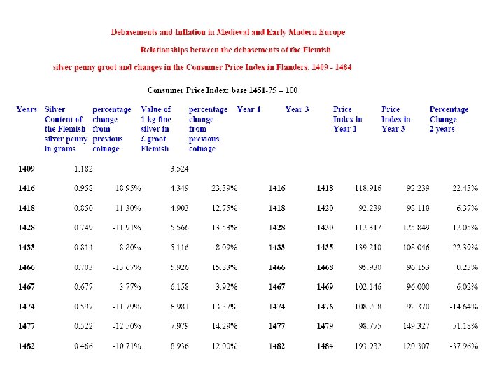
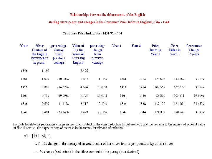
Quantity Theories of Money - 7 • -d) possible exception: coinage debasements, increasing M, may also increase V (= fall in k): as a ‘flight from money’ into real assets • - but not during Henry VIII’s ‘Great Debasement’ (1542 -51) • - also not so during 15 th century Flemish debasements • (7) Changes in Friedman’s ‘y’ (NNI = NNP): ‘real’ variable • - an endogenous or exogenous variable? • - what was the impact of population growth and technological changes on ‘y’?

Quantity Theories of Money - 8 • (8) Monetarists and Keynesian views on V and k (V = 1/k): • - Monetarists: believe that V (1/k) is fixed or relatively stable, at least in the short-run • - Keynesians: believe the opposite: • that V is very flexible in the short run • - Keynesians also believe that k = 1/V is very responsive to changes in interest rates: that it will rise when interest rates fall

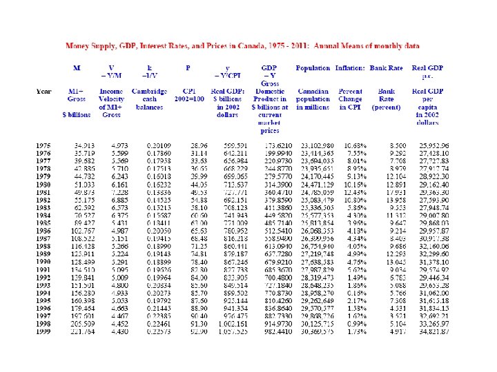
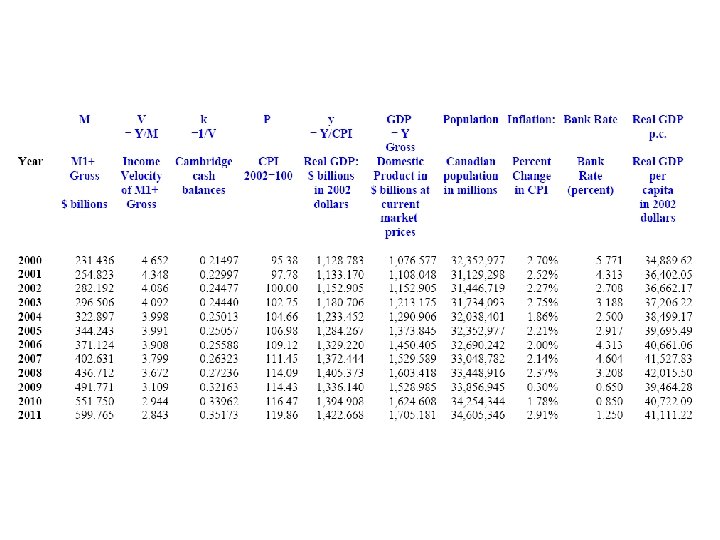
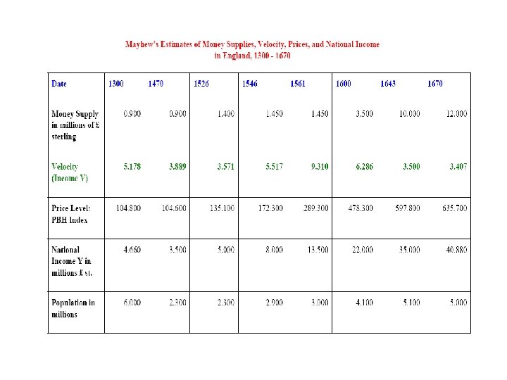
Recent Canadian Monetary Experience - 1 • (1) Behaviour of V = 1/k: 1975 to 2011 • - V (based on M as M 1+ Gross): • - has ranged from a low of 2. 843 in 2011 (k = 0. 342) to the previous high of 7. 228 in 1981 (k = 0. 138) • - V had risen from 1975 (and earlier) to this 1981 peak: • - Note the considerable expansion in the money supply (M 1+) -- and Keynes proposition: that V will fall (‘k’with a rise in M: also seen in Mayhew’s table).

Recent Canadian Monetary Experience - 2 • 2) Cambridge ‘k’ and the Bank Rate: • - Keynes also predicted that ‘k’ will vary inversely with the bank rate: • Why? Because holding cash balances has an opportunity cost: foregoing investment income • in 1981, Bank Rate was at its high – 17. 931% and Cambridge ‘k’ was at that low of 0. 138 • - in 2010: Bank Rate = 0. 850% and k = 0. 340 (but 0. 352 in 2011, when Bank Rate rose to 1. 250%)

Recent Canadian Experience - 3 • (3) Relationship between M and Price level • a) Money supply (M 1+): grown from $34. 913 billion in 1975 to $599. 765 billion in 2011: a 17. 178 fold increase (= 1617. 88%) • b) The CPI (2002=100): has increased from 28. 96 in 1975 to 119. 86 in 2011: only a 4. 138 fold increase (= 313. 88%) • c) Real GDP (2002 dollars): has grown from $599. 591 billion in 1975 to $1, 422. 668 billion in 2011 (+137. 27%) • d) Population: grown from 23. 102 million in 1975 to 34. 605 million in 2011 (1. 498 fold increase = 49. 79%)

Recent Canadian Experience - 3 4) Conclusions on the Quantity Theory: a) the expansion in M was offset by: - a fall in V (= rise in ‘k’) - an expansion in y = NNP (here: real GDP b) importance of population growth: contributed to growth in GDP, thus offsetting inflationary force of Δ M • c) Growth in Real GDP per capita ($2002): from $25, 953 in 1975 to $41, 111 in 2011 (1. 584 fold increase = 58. 40% increase) • • •

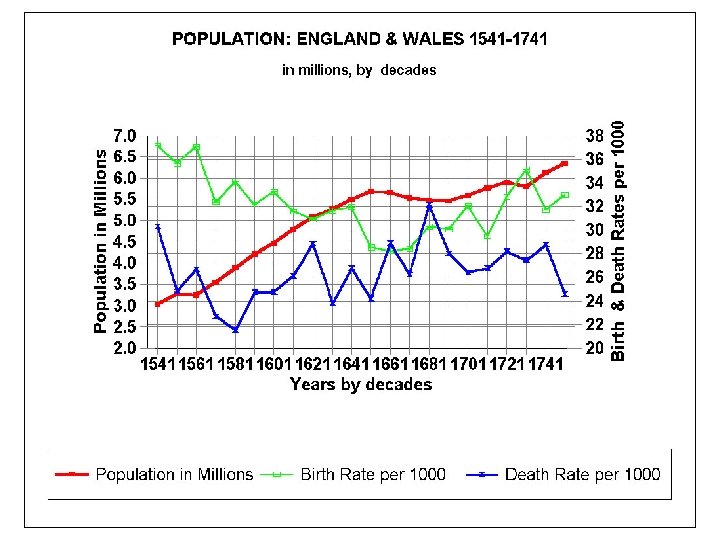
The Role of Population in the Price Revolution era (1520 – 1650) - 1 • (1) Basic premise of the Real School is a fallacy: that population growth itself ‘caused’ the Price Revolution: • a) Note: inflation began before the demographic recovery: • - inflation: from about 1515 (in England & Low Countries) • - demographic growth: from the 1520 s (in same regions) • b) this Real model confuses micro- and macro-economics: • i) Yes: population growth can produce an increase in individual, relative prices -- for grains, lumber, fuels, etc. , • ii) But: population growth by itself cannot cause a rise in the general price level: in the CPI

The Role of Population in the Price Revolution era (1520 – 1650) - 2 • c) micro-economics: rise in prices of necessities (whose production subject to diminishing returns) would lead, in context of family budget constraints, to reduced demand relative fall (real fall) in prices of other commodities • d) key factor: differences in supply & demand elasticities, in the longer run (see graphs)

Relative price changes with population growth

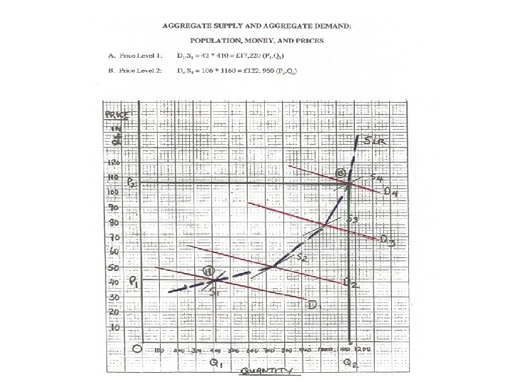
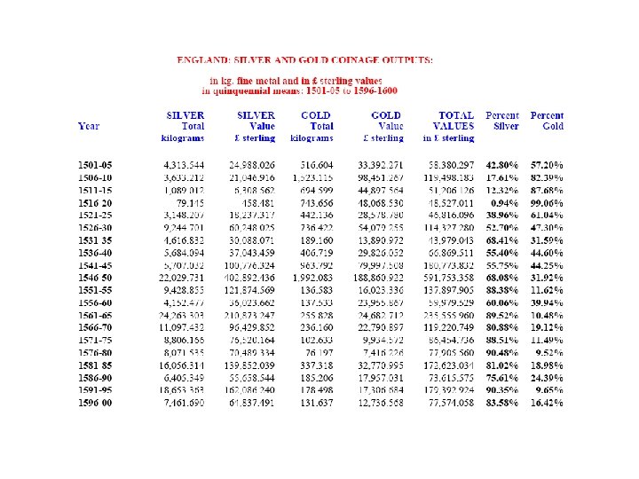
The Role of Population in the Price Revolution (3) • (2) Keynesian Aggregate Demand: Population growth and inflation: • a) If we shift the aggregate demand curve upwards, on basis of population growth, and we see a rise in the price level, what are we missing in this model? • b) the fact that prices in the model are measured in terms of a silver-based money-of-account • i) note that with a rise in price level from P(1) to P(2), the value of PQ(1) rises from £ 17, 220 to £ 122, 960 for the value of PQ(2): • ii) where does all that extra money come from: an increase in M or an increase in V, or both? ?

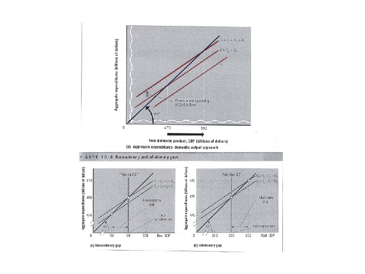
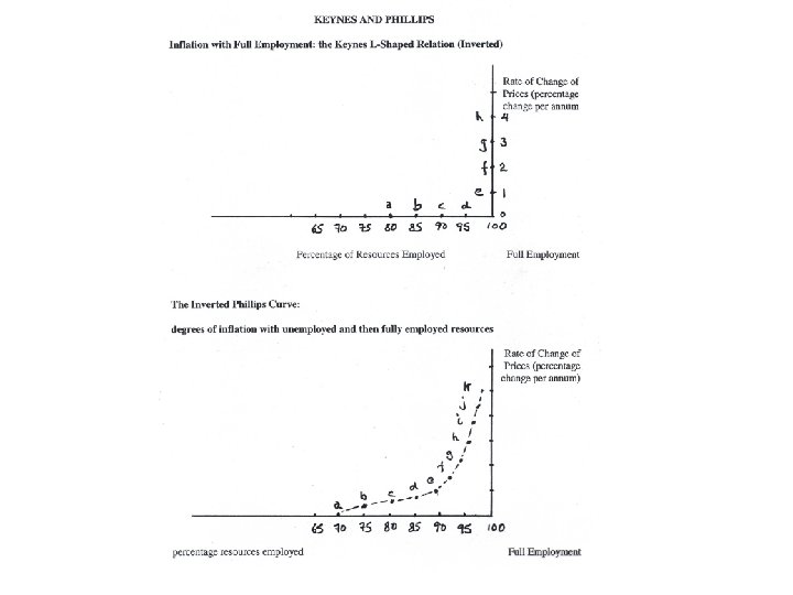
The Role of Population in the Price Revolution (4) • (3) The Phillips Curve (1958 article): demonstrating a negative correlation between changes in unemployment rates and the price level, 1861 - 1913 • the closer an economy reached full employment, the higher rose the price level • - conversely: the higher the unemployment, the more stable was the price level • note difference from the Keynesian L-shaped national income diagram: Y = C+I+G+(X-M)

The Phillips Curve: relating unemployment and money wage rates

Keynes: the General Theory (1936) • It is probable that the general level of prices will not rise very much as output increases, so long as there available efficient unemployed resources of every type. • But as soon as output has increased sufficiently to begin to reach the ‘bottle necks’, there is likely to be a sharp rise in the prices of certain commodities.

The Role of Population in the Price Revolution (5) (1) The potential effects on population growth on money, output, and prices: • a) 0 n Supply Side: • i) fuller employment of existing resources • ii) diminishing returns and rising marginal costs in agriculture and natural-resource (extraction) industries

The Role of Population in the Price Revolution (6) (1) The potential effects on population growth on money, output, and prices: cont’d b) On the Demand Side: • i) increased demand for money (increased ‘k’) reduce inflationary impact from Δ M • ii) changes in structure of demand with more urbanization (Goldstone effect) • iii) changes in population’s age pyramid larger families with more children per adult further changes in aggregate demand (Lindert effect)

The Role of Population in the Price Revolution (7) • (2) The Goldstone Velocity Theory of Inflation: • -a) the case of England: rapid population growth produced disproportionate urbanization, with far more complex, more fully monetized market structures (agriculture + industry) • accompanied by growth of commercial + financial institutions: much more credit used • “in occupationally specialized linked networks, the potential velocity of circulation of coins grows as the square of the size of the network”

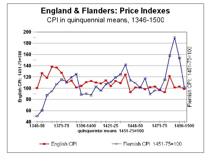
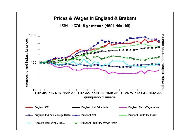
The Role of Population in the Price Revolution (8): Velocity A • b) Major Problems with the Goldstone thesis: • i) in both England Low Countries, Price Revolution began before 1520 (ca. 1515) – before any signs of significant population growth (as stressed earlier) • ii) Note the similarity of the degree of inflation in both countries: • but Low Countries had become far more urbanized, commercialized, and more advanced in these more complex networks a century before England

The Role of Population in the Price Revolution (9): Velocity A • b) Major Problems with the Goldstone thesis: • iv) pretends that velocity is a demographic variable: • it is of course a monetary variable – V = 1/k. • iii) ignores all the evidence on vast increases in the money supply in both countries: as presented in last lecture, for England & Low Countries

The Role of Population in the Price Revolution (10): Velocity B • (3) The Lindert Velocity Model: • How population growth may have led to an increase in the income velocity of money: • a) by raising the cost of living: especially in food prices + fuel reduction in demand for idle balances, inducing dishoarding • b) by increasing family size and thus ratio of dependent children (non-earners) to adults similarly reducing cash balances, inducing dishoarding • c) but how long could this have been sustained?

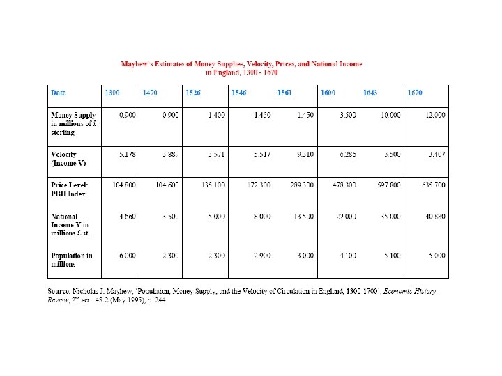
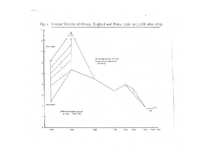
The Role of Population in the Price Revolution (11): Velocity C • (4) Nicholas Mayhew on Income Velocity of Money in England: • a) agrees with Lindert, Goldstone, Miskimin: that the income velocity of money (V) rose during the Price Revolution era (1520 – 1650) • b) But, before and after, he agrees with Keynes: that increases in the money supply fall in income velocity of money = rise in ‘k’: primarily because of a fall in real interest rates (Keynes LP schedule) • c) Changed composition of the coinage supply: • shift from gold to silver, with a far higher transactions & income velocity for silver coins:

Monetary, Demographic, and Price Trends, 1348 - 1750 • • • (1) 1348 – 1370 s: Era of the Black Death - severe demographic crises & rapid population decline (40%) - but also severe inflation (2) 1370 s – 1490 s: late-medieval ‘Great Depression’: second phase - continued demographic decline & stagnation - two ‘bullion famines’ severe deflation (except during major wars + debasement) (3) 1490 s – 1520 s: monetary expansion, commercial-economic recovery, but no inflation (4) 1520 s – 1640 s: era of Price Revolution: monetary, economic, then demographic expansion, with sustained inflation (5) 1640 s – 1740 s: era of the ‘General Crisis’ with: - monetary contraction deflation (except during wartime) - demographic decline or stagnation

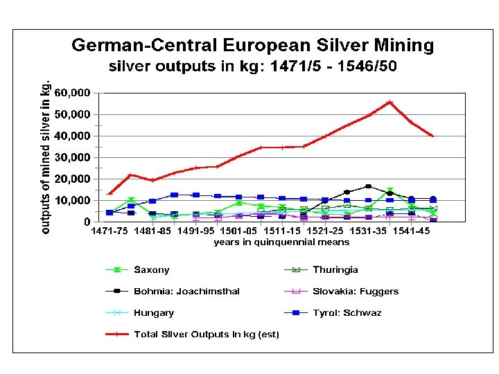
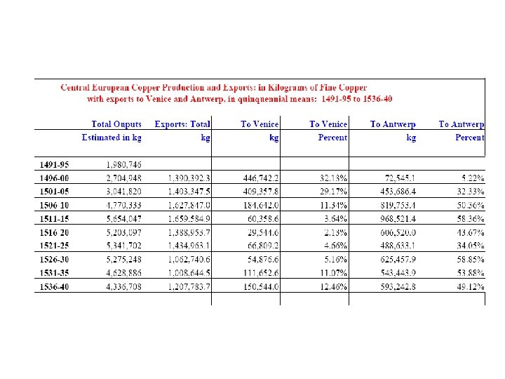
Money, Population, Prices: before and during the Price Revolution era • (1) the South German-Central European mining boom: c. 1460 – c. 1540: • -a) ended late-medieval ‘bullion famines’ -- with a five -fold expansion in European silver + copper supplies • - b) rise of the Antwerp Market, from 1460 s: based on tripod of English woollens, German metals (& banking), Portuguese Asian spices • c) note that this monetary and economic expansion well preceded the demographic recovery & expansion (from 1520 s • in both England Low Countries (not before 1520) • if somewhat earlier in Italy and South Germany

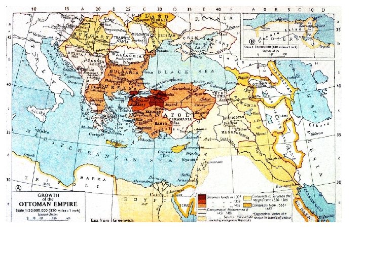
Money, Population, Prices: before and during the Price Revolution era (2) • (2) Why was there no Price Revolution from 1460 s to ca. 1520? • a) Major expansion in Central European mining came after 1516: opening of Joachimsthal silver mines (Bohemia) • b) Venetian wars with Turks from 1490 s: curbed trade with & silver exports to Levant • - 1517: Ottoman conquest of Mamluk Egypt and Syria + the new Portuguese trade with Asia: severe drop in Venetian silver + copper exports more German silver and copper going to Antwerp market • - but somewhat offset by Portuguese silver exports to Asia • c) changes in aggregate supplies: elastic before 1510?

Money, Population, Prices: before and during the Price Revolution era (3) • c) Lessons from the Philips curve: • - there were so many unemployed resources (land, labour, capital) from the late-phase of the ‘Great Depression’ era, that economic recovery & growth took place with elastic supplies of inputs, without rising MC so no price increases • that ‘bottlenecks’ and rising marginal costs not encountered before ca. 1515 -1520: still much ‘slack’ in the economy • - problem: no significant population growth in NW Europe before the 1520 s

Money & Population during the Price Revolution era, c. 1520 – 1640 (4) • (3) Money supplies: more rapid expansion • a) height of the Central European mining boom: ca. 1520 – ca. 1540 • b) influx of gold, then silver from Spanish America, especially from 1550 s • c) coinage debasements: England + Low Countries: but not in Spain • (2) Credit: financial revolution in negotiable credit instruments + negotiable public debts: from 1520 s • (3) Population growth: from the 1520 s: effects of Δ urbanization on income velocity of money?

Monetary Approach to Balance of Payments (1) • 1) Read lectures: for today and last week • 2) Problem 1: suppositions of Classical School on international trade and inflation • a) favourable balance of trade (export revenues > imports) bullion influx ΔM inflation • b) unfavourable trade balance bullion outflow fall in M deflation • 3) Problem 2: Inflation was European-wide, but • a) Not all countries could have had a continuous favourable trade balances • b) especially with Δ bullion outflows in trade with Levant, southern Asia, Baltic zone

Monetary Approach to Balance of Payments (2) • (4) Solution: Monetary Approach to Balance of Payments: Prof. Harry Johnson • a) world bullion stocks determine overall world price level (in terms of silver) • b) ‘law of one price’ in international trade (arbitrage): will establish same commensurate price level in each country • c) each country’s money supply adjusts to accommodate that increased price level

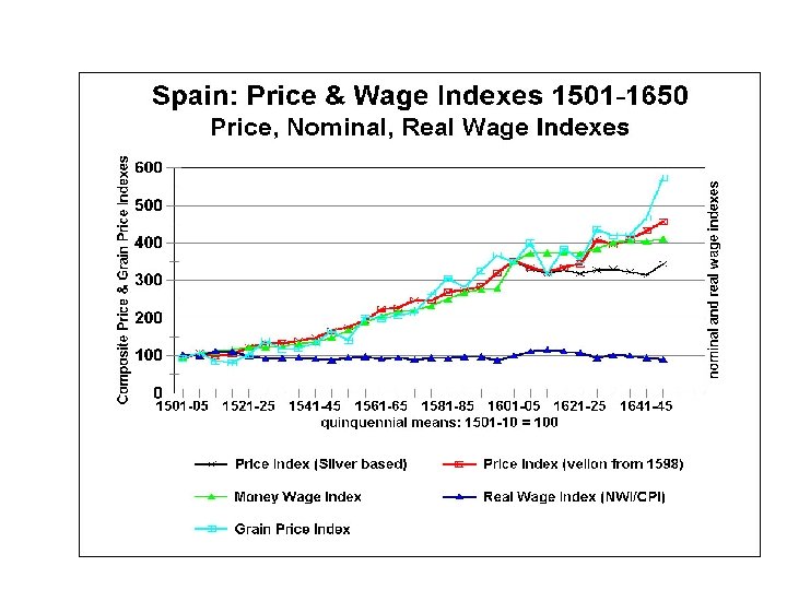
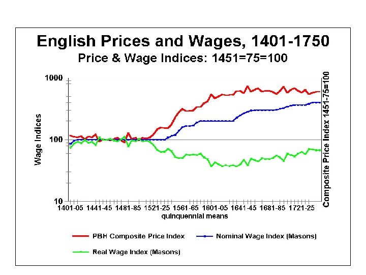
Consequences of Inflation: Impact on Factor Costs of Production - 1 • (1) Hamilton’s Thesis of ‘Profit Inflation’: on lagging real wages and 16 th century industrialization • a) his most famous role: Quantity Theory of money in explaining Price Revolution • b) also important for his thesis on the origins of modern industrial capitalism • - contended that during the Price Revolution, wages lagged behind consumer prices, providing entrepreneurs with growing profits • - argued that industrial entrepreneurs invested those extra profits in more capital-intensive, larger scale forms of industry

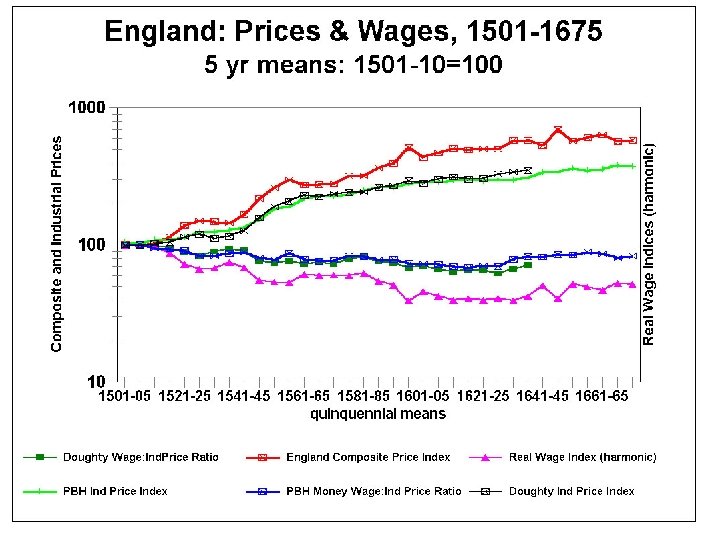
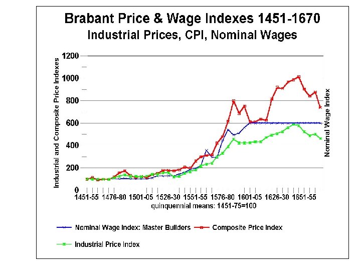
Consequences of Inflation: Impact on Factor Costs of Production - 2 • -c) that this was much more true of England than of Spain or France: hence a major reason why England became homeland of the Industrial Revolution • -d) his ‘profit inflation’ thesis warmly endorsed by J. M. Keynes (who actually coined the phrase). • - e) Note: historically, during periods of inflation, wages do indeed lag behind consumer prices (irrespective of demographic changes): so that real wages necessarily fall [RWI = NWI/CPI]

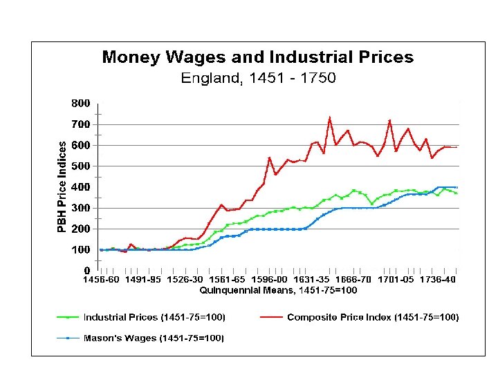
Consequences of Inflation: Impact on Factor Costs of Production - 3 • f) problems with Hamilton’s ‘profit inflation’ thesis: • i) what prices? Hamilton never clear on this crucial issue: the CPI, agricultural or industrial prices? • if the CPI, heavily weighted with food prices, rose, how would falling real wages benefit entrepreneurs? [RWI = NWI/CPI] • - rising food + fuel prices would, with budget constraints, curb much of the market demand for industrial goods from wage earners • - though impact would have been somewhat offset by rising real incomes for agricultural producers

Consequences of Inflation: Impact on Factor Costs of Production - 4 • f) problems with Hamilton’s ‘profit inflation’ thesis: • ii) the true issue must be: did industrial wages lag behind the wholesale prices for the same industrial products? • iii) even if wages did lag, did entrepreneurs encounter other rising input or factor costs during Price Revolution era? • iv) Even if industrial entrepreneurs did earn increased profits, why would they choose to invest them in more capital intensive forms of larger scale industry, if labour was becoming relatively cheaper?

Consequences of Inflation: Impact on Factor Costs of Production (5) • (2) Land Rents: did they rise with agricultural prices? • - English agriculture: customary (servile) rents did not rise: fixed by custom, in money-of-account terms • - Agriculture & Enclosures: • - incentives for landlords to evict customary tenants, to recapture ‘economic rent’ on land, with rising grain prices • - leasehold lands: • - rents were fixed for the period of contractual leases, • so that those renting such lands (farmers, industrial entrepreneurs) benefited from rising prices of products produced on those leasehold lands

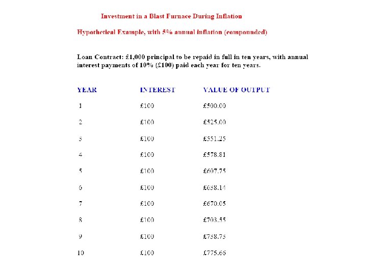
Consequences of Inflation: Impact on Factor Costs of Production (6) • (3) Other land-based factor costs: rising costs of wood-based fuels in particular led John Nef (Hamilton’s Chicago colleague) to offer his alternative thesis on origins of modern industrial capitalism in Price Revolution era, in Tudor-Stuart England • - we will deal with the Nef thesis in the final lecture on Tudor Stuart ‘Industrial Revolution’ • (4) Capital and Interest: did inflation cheapen capital costs? YES: it did cheapen the costs of previously borrowed capital

Deflation during the ‘General Crisis’ era, c. 1650 – c. 1740: 1 • (1) Deflation from the 1650 s to the 1740 s: except for the war-torn 1690 s • (2) Possible Causes? last day’s lecture: • a) monetary contraction: as outflows of silver to Baltic, Levant, East Asia exceeded the declining influx from the Americas • b) demographic contractions or slumps • c) declines in the income velocity of money?

Deflation during the ‘General Crisis’ era, c. 1650 – c. 1740: 2 • 3) Problems: with and from deflation: • a) raised the real and relative factor costs of production: • i) wage stickiness: nominal wages remain flat real wages rise with deflation • ii) land rent contracts: fixed by leases for many years (up to 99 years): fixed nominal rents thus rising real burden of rent with deflation • iii) interest rates by longer-term contracts: similar situation with nominal rents rising real rates

Deflation during the ‘General Crisis’ era, c. 1650 – c. 1740: 3 • b) deflation hurts credit and curbs investment • i) fear of non-repayment: paper credit generally contracts more than the coined money supplies • ii) reluctance to borrow: with anticipated rises in real interest rates • iii) economic pessimism: reduces incentives to produce and invest