Macroeconomic Theory Chapter 7 Exogenous Growth Theory Macroeconomic

Macroeconomic Theory Chapter 7 Exogenous Growth Theory Macroeconomic Theory Prof. M. El-Sakka CBA. Kuwait University

o Long run economic growth determines how living standards o o o change. This chapter introduces exogenous growth theory, beginning with the Solow-Swan model. The role of capital, savings, population growth and technological progress in determining the equilibrium levels of output per worker in the economy is also elaborated. There are two key concepts in growth theory, the steady state or balanced growth, and the transitional dynamics (what happens when steady state is disturbed). The growth model in the long run is characterized as one of steady state growth or as a balanced growth path in which output and employment grow at constant proportional rates and in which net savings (and investment) is a constant share of output, and the growth rate of output per-capita is zero. A key characteristic of the Solow-Swan model is that technological progress is an exogenous force. Macroeconomic Theory Prof. M. El-Sakka CBA. Kuwait University

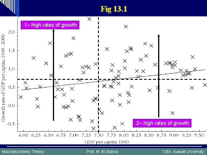
o Key concepts in the discussion of income disparities are those of absolute and conditional convergence. o A much weaker notion of diversion is labeled conditional divergence; countries would not be expected to converge to the same living standards unless they are similar in important respects, such as having the same saving rate. This means that poor countries will not catch up and achieve the living standards of the rich countries unless they are able to change the determinants of their steady state. o Although the Solow-Swan model provides the foundation for growth theory, there has been much work on developing models in which the growth of living standards is endogenous, rather than the result of exogenous growth. Macroeconomic Theory Prof. M. El-Sakka CBA. Kuwait University

Fig 13. 1 1– high rates of growth 2– high rates of growth Macroeconomic Theory Prof. M. El-Sakka CBA. Kuwait University

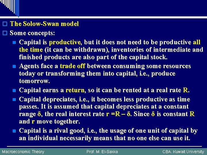
o The Solow-Swan model o Some concepts: n n n Capital is productive, but it does not need to be productive all the time (it can be withdrawn), inventories of intermediate and finished products are also part of the capital stock. Agents face a trade off between consuming some resources today or transforming them into capital, i. e. , produce tomorrow. Capital earns a return, so it can be rented at a real rate R. Capital depreciates, i. e. , it becomes less productive as time passes. It is assumed that capital depreciates at a constant range δ, the real interest rate r =R – δ. Since δ is constant R and r move together. Capital is a rival good, i. e. , the usage of one unit of capital by an individual necessarily means that no one else can use it. Macroeconomic Theory Prof. M. El-Sakka CBA. Kuwait University

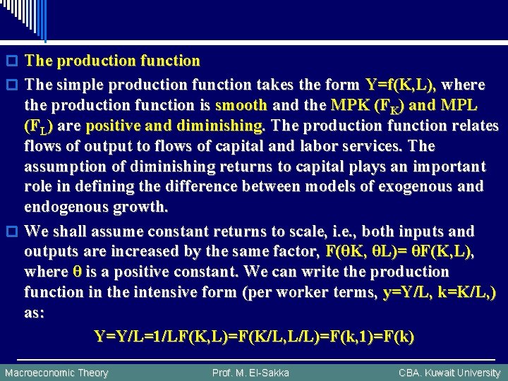
o The production function o The simple production function takes the form Y=f(K, L), where the production function is smooth and the MPK (FK) and MPL (FL) are positive and diminishing. The production function relates flows of output to flows of capital and labor services. The assumption of diminishing returns to capital plays an important role in defining the difference between models of exogenous and endogenous growth. o We shall assume constant returns to scale, i. e. , both inputs and outputs are increased by the same factor, F(θK, θL)= θF(K, L), where θ is a positive constant. We can write the production function in the intensive form (per worker terms, y=Y/L, k=K/L, ) as: Y=Y/L=1/LF(K, L)=F(K/L, L/L)=F(k, 1)=F(k) Macroeconomic Theory Prof. M. El-Sakka CBA. Kuwait University

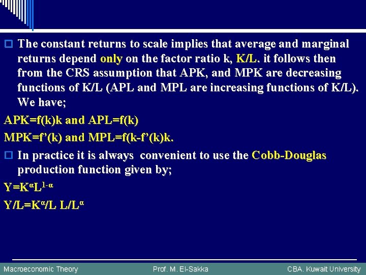
o The constant returns to scale implies that average and marginal returns depend only on the factor ratio k, K/L. it follows then from the CRS assumption that APK, and MPK are decreasing functions of K/L (APL and MPL are increasing functions of K/L). We have; APK=f(k)k and APL=f(k) MPK=f’(k) and MPL=f(k-f’(k)k. o In practice it is always convenient to use the Cobb-Douglas production function given by; Y=KαL 1 -α Y/L=Kα/L L/Lα Macroeconomic Theory Prof. M. El-Sakka CBA. Kuwait University

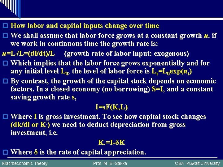
o How labor and capital inputs change over time o We shall assume that labor force grows at a constant growth n. if we work in continuous time the growth rate is: n=L. /L=(dl/dt)/L (growth rate of labor input: exogenous) o Which implies that the labor force grows exponentially and for any initial level L 0, the level of labor force is Lt=L 0 exp(nt) o By contrast, the growth of the capital stock depends on economic factors. In a closed economy (no borrowing) S=I, and a constant saving growth rate s, I=s. F(K, L) o Where I is gross investment. To see how capital stock changes (dk/dl or K. ) we need to deduct depreciation from gross investment, i. e. K. =I-δK o Where δ is the rate of capital appreciation. Macroeconomic Theory Prof. M. El-Sakka CBA. Kuwait University

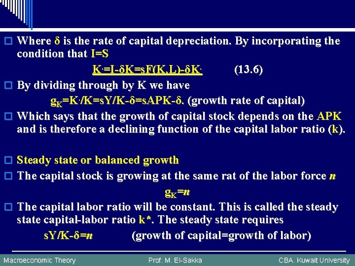
o Where δ is the rate of capital depreciation. By incorporating the condition that I=S K. =I-δK=s. F(K, L)-δK. (13. 6) o By dividing through by K we have g. K=K. /K=s. Y/K-δ=s. APK-δ. (growth rate of capital) o Which says that the growth of capital stock depends on the APK and is therefore a declining function of the capital labor ratio (k). o Steady state or balanced growth o The capital stock is growing at the same rat of the labor force n g. K=n o The capital labor ratio will be constant. This is called the steady state capital-labor ratio k*. The steady state requires s. Y/K-δ=n (growth of capital=growth of labor) Macroeconomic Theory Prof. M. El-Sakka CBA. Kuwait University

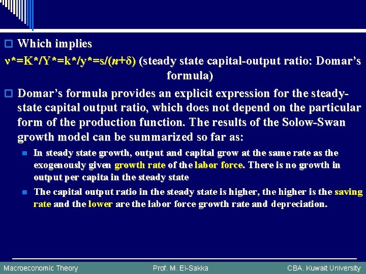
o Which implies ν*=K*/Y*=k*/y*=s/(n+δ) (steady state capital-output ratio: Domar’s formula) o Domar’s formula provides an explicit expression for the steadystate capital output ratio, which does not depend on the particular form of the production function. The results of the Solow-Swan growth model can be summarized so far as: n n In steady state growth, output and capital grow at the same rate as the exogenously given growth rate of the labor force. There is no growth in output per capita in the steady state The capital output ratio in the steady state is higher, the higher is the saving rate and the lower are the labor force growth rate and depreciation. Macroeconomic Theory Prof. M. El-Sakka CBA. Kuwait University

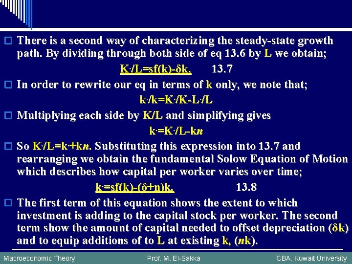
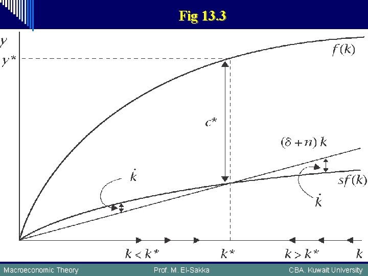
o There is a second way of characterizing the steady-state growth o o path. By dividing through both side of eq 13. 6 by L we obtain; K. /L=sf(k)-δk. 13. 7 In order to rewrite our eq in terms of k only, we note that; k. /k=K. /K-L. /L Multiplying each side by K/L and simplifying gives k. =K. /L-kn So K. /L=k. +kn. Substituting this expression into 13. 7 and rearranging we obtain the fundamental Solow Equation of Motion which describes how capital per worker varies over time; k. =sf(k)-(δ+n)k. 13. 8 The first term of this equation shows the extent to which investment is adding to the capital stock per worker. The second term show the amount of capital needed to offset depreciation (δk) and to equip additions of to L at existing k, (nk). Macroeconomic Theory Prof. M. El-Sakka CBA. Kuwait University

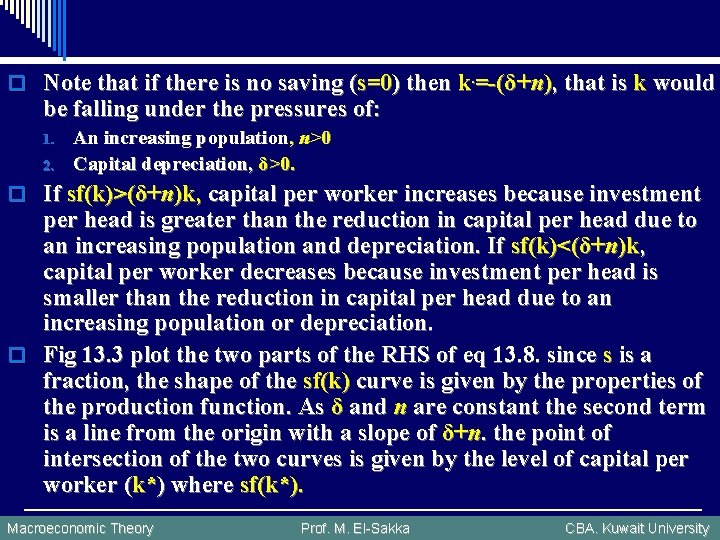
o Note that if there is no saving (s=0) then k. =-(δ+n), that is k would be falling under the pressures of: 1. 2. An increasing population, n>0 Capital depreciation, δ>0. o If sf(k)>(δ+n)k, capital per worker increases because investment per head is greater than the reduction in capital per head due to an increasing population and depreciation. If sf(k)<(δ+n)k, capital per worker decreases because investment per head is smaller than the reduction in capital per head due to an increasing population or depreciation. o Fig 13. 3 plot the two parts of the RHS of eq 13. 8. since s is a fraction, the shape of the sf(k) curve is given by the properties of the production function. As δ and n are constant the second term is a line from the origin with a slope of δ+n. the point of intersection of the two curves is given by the level of capital per worker (k*) where sf(k*). Macroeconomic Theory Prof. M. El-Sakka CBA. Kuwait University

Fig 13. 3 Macroeconomic Theory Prof. M. El-Sakka CBA. Kuwait University

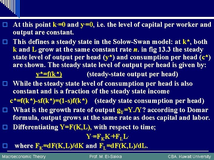
o At this point k. =0 and y. =0, i. e. the level of capital per worker and output are constant. o This defines a steady state in the Solow-Swan model: at k*, both k and L grow at the same constant rate n. in fig 13. 3 the steady state level of output per head (y*) and consumption per head (c*) are shown. The steady state level of output per head is given by: y*=f(k*) (steady-state output per head) o While the steady state level of consumption per head is also constant and is a fraction of the steady state income c*=f(k*)-sf(k*)=(1 -s)f(k*) (steady state consumption per head) o What is the growth rate of output g. Y=Y. /Y? according to Domar formula, output grows at the same rate as does capital and labor. o Differentiating Y=F(K, L), with respect to time; Y. =FKK. +FLL. o where FK=d. F(K, L)/d. K and FL=d. F(K, L)/d. L. Macroeconomic Theory Prof. M. El-Sakka CBA. Kuwait University

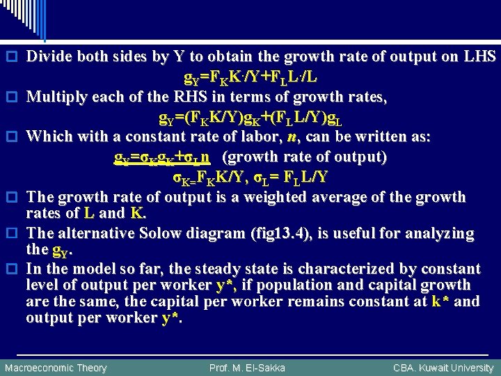
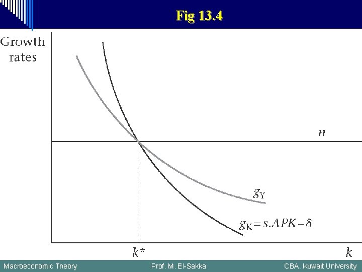
o Divide both sides by Y to obtain the growth rate of output on LHS o o o g. Y=FKK. /Y+FLL. /L Multiply each of the RHS in terms of growth rates, g. Y=(FKK/Y)g. K+(FLL/Y)g. L Which with a constant rate of labor, n, can be written as: g. Y=σKg. K+σLn (growth rate of output) σK=FKK/Y, σL= FLL/Y The growth rate of output is a weighted average of the growth rates of L and K. The alternative Solow diagram (fig 13. 4), is useful for analyzing the g. Y. In the model so far, the steady state is characterized by constant level of output per worker y*, if population and capital growth are the same, the capital per worker remains constant at k* and output per worker y*. Macroeconomic Theory Prof. M. El-Sakka CBA. Kuwait University

Fig 13. 4 Macroeconomic Theory Prof. M. El-Sakka CBA. Kuwait University

o The intuition for this result is clear: diminishing returns to K ensure that extra unit of K per worker produce less and less; at the same time depreciation does not diminish. Eventually all savings must will be deployed to replace the existing capital, i. e. , when sf(k*) cuts the (δ+n)k line in fig 13. 3, the point at which the economy will be in eq with k. =0. o o Transitional dynamics: what happens out of equilibrium? In fig 13. 3 when capital labor ratio is below the steady state, capital intensity will increase and vice versa. The economy will adjust until k=k*. It is useful to present the model in a slightly different way. Consider g. K=k. /k, the growth rate of capital per worker. Divide eq 13. 8 by k to obtain gk=sf(k)/k-(δ+n) =s. APK-(δ+n) Macroeconomic Theory Prof. M. El-Sakka CBA. Kuwait University

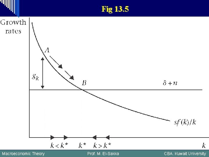
o The two components of the RHS are plotted in fig 13. 5. in the steady state when k=k*, sf(k*)/k*=δ+n, thus the growth rate of capital per worker is given by the vertical distance between the tow curves. Given the growth rate of L, n, capital stock per worker also grows. The economy moves from A to B. similarly, for high k, capital stock per worker will decline. o Following the same procedure we used for working out the growth rate of Y, we have gy=(MPK/APK)gk=σKg. K (growth rate of output per head) o Where with competitive markets, σK is capital’s share of output and is positive and less than one. In the steady state, the equation still holds because gy=gk=0 Macroeconomic Theory Prof. M. El-Sakka CBA. Kuwait University

Fig 13. 5 Macroeconomic Theory Prof. M. El-Sakka CBA. Kuwait University

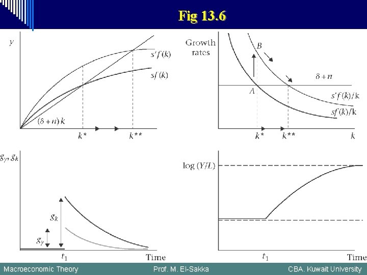
o Policy experiment 1: a rise in the saving rate o At time t 1, there is an exogenous rise in the saving rate, fig 13. 6 traces the impact of this shock and show k and y adjust as the economy moves to a new steady state. We only observe a positive growth rates in per worker variables if the economy experiences a parameter shift. Once the system returns to its steady state we are back on the balanced growth path with zero growth of output per capita. o Along with the rise in capital per worker and productivity, there is a rise in the capital output ratio. This means that the faster capital stock growth generated by the higher savings rate fades away as depreciation eventually swallows up all the additional investment effort. Macroeconomic Theory Prof. M. El-Sakka CBA. Kuwait University

Fig 13. 6 Macroeconomic Theory Prof. M. El-Sakka CBA. Kuwait University

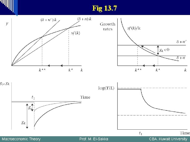
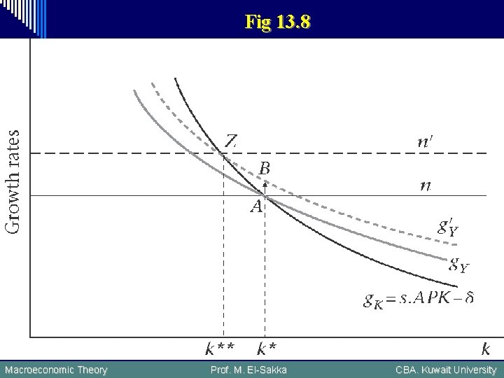
o Policy experiment 2: a rise in the population growth rate. o Population growth suddenly and permanently goes up due to an exogenous change in fertility. Fig 13. 7 shows the impact of this shock on the system, it traces how k and y adjust to the new steady state. At k** capital per worker and output per worker is lower than at t 1, capital intensity declines. o What happens to the growth rate of output in this economy? To see this we use alternative Solow diagram in fig 13. 8. Macroeconomic Theory Prof. M. El-Sakka CBA. Kuwait University

Fig 13. 7 Macroeconomic Theory Prof. M. El-Sakka CBA. Kuwait University

Fig 13. 8 Macroeconomic Theory Prof. M. El-Sakka CBA. Kuwait University

o These experiments leave an open question of what generates the type of sustained growth documented in chapter 1. the model can account for this by either o The response of very long adjustment periods as the economy transits from one steady state to another o The presence of repeated shocks, e. g. , a steadily rising savings share or a steadily falling population growth rate. Macroeconomic Theory Prof. M. El-Sakka CBA. Kuwait University

o Solow growth accounting: measuring the impact of technology Macroeconomic Theory Prof. M. El-Sakka CBA. Kuwait University