Variational Methods for Graphical Models Micheal I Jordan

Variational Methods for Graphical Models Micheal I. Jordan Zoubin Ghahramani Tommi S. Jaakkola Lawrence K. Saul Presented by: Afsaneh Shirazi

Outline • • Motivation Inference in graphical models Exact inference is intractable Variational methodology – Sequential approach – Block approach • Conclusions 2

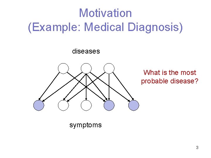
Motivation (Example: Medical Diagnosis) diseases What is the most probable disease? symptoms 3

Motivation • We want to answer some queries about our data • Graphical model is a way to model data • Inference in some graphical models is intractable (NP-hard) • Variational methods simplify the inference in graphical models by using approximation 4

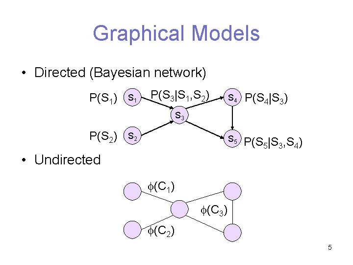
Graphical Models • Directed (Bayesian network) P(S 1) S 1 P(S 3|S 1, S 2) S 4 P(S 4|S 3) S 5 P(S 5|S 3, S 4) S 3 P(S 2) S 2 • Undirected (C 1) (C 3) (C 2) 5

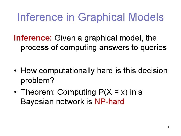
Inference in Graphical Models Inference: Given a graphical model, the process of computing answers to queries • How computationally hard is this decision problem? • Theorem: Computing P(X = x) in a Bayesian network is NP-hard 6

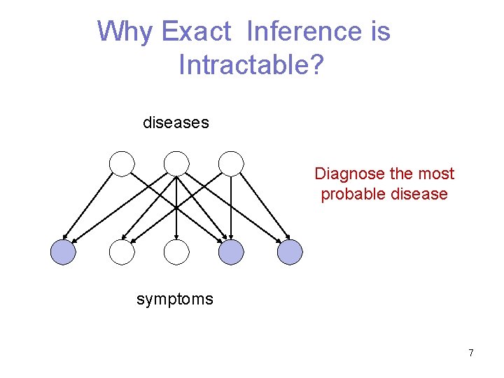
Why Exact Inference is Intractable? diseases Diagnose the most probable disease symptoms 7

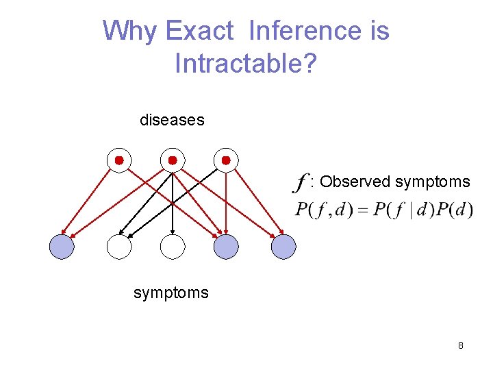
Why Exact Inference is Intractable? diseases : Observed symptoms 8

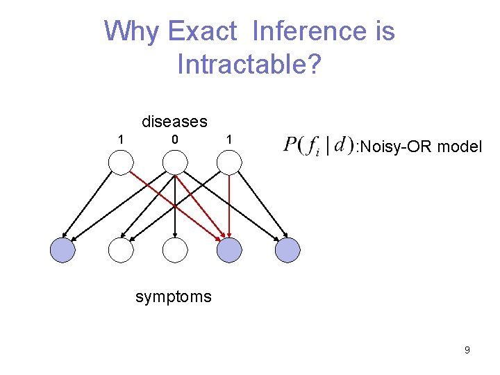
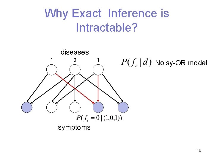
Why Exact Inference is Intractable? diseases 1 0 1 : Noisy-OR model symptoms 9

Why Exact Inference is Intractable? diseases 1 0 1 : Noisy-OR model symptoms 10

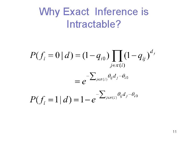
Why Exact Inference is Intractable? 11

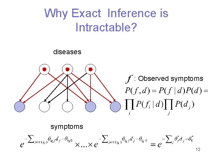
Why Exact Inference is Intractable? diseases : Observed symptoms 12

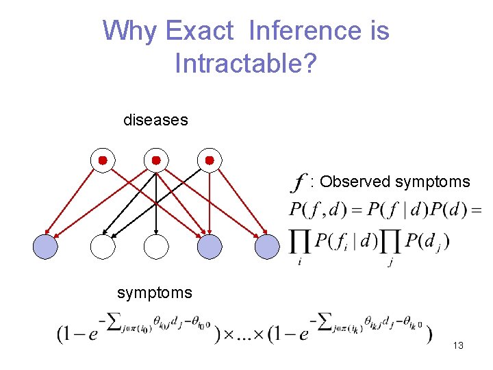
Why Exact Inference is Intractable? diseases : Observed symptoms 13

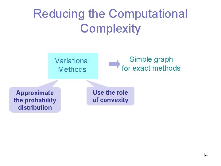
Reducing the Computational Complexity Variational Methods Approximate the probability distribution Simple graph for exact methods Use the role of convexity 14

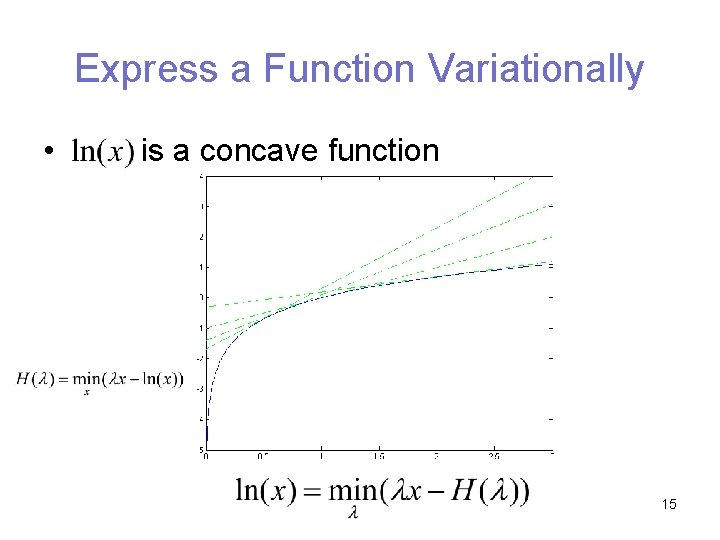
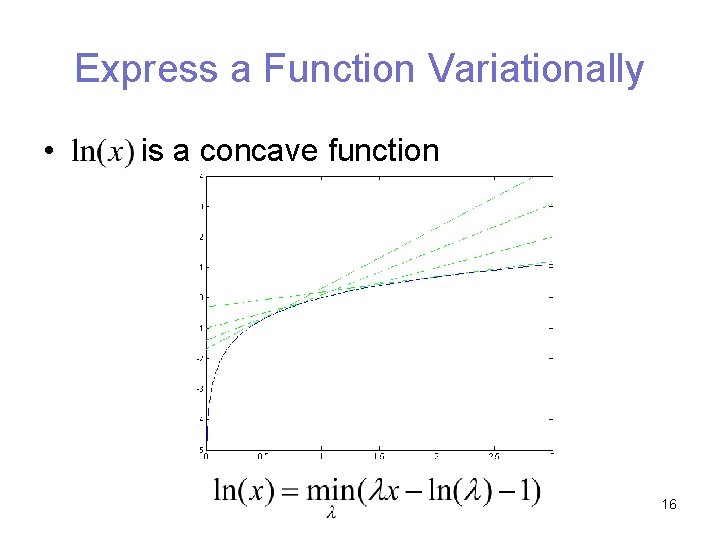
Express a Function Variationally • is a concave function 15

Express a Function Variationally • is a concave function 16

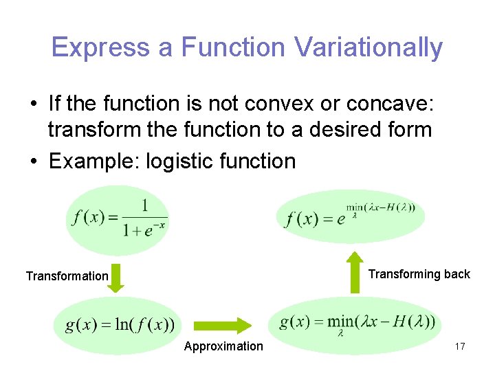
Express a Function Variationally • If the function is not convex or concave: transform the function to a desired form • Example: logistic function Transforming back Transformation Approximation 17

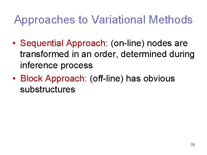
Approaches to Variational Methods • Sequential Approach: (on-line) nodes are transformed in an order, determined during inference process • Block Approach: (off-line) has obvious substructures 18

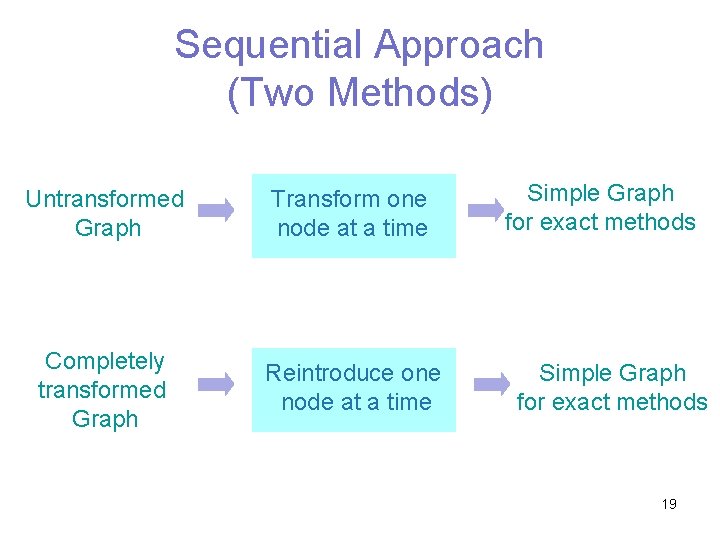
Sequential Approach (Two Methods) Untransformed Graph Transform one node at a time Completely transformed Graph Reintroduce one node at a time Simple Graph for exact methods 19

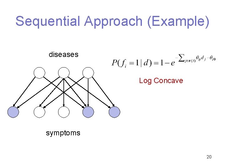
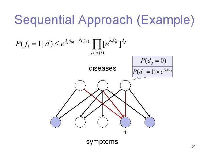
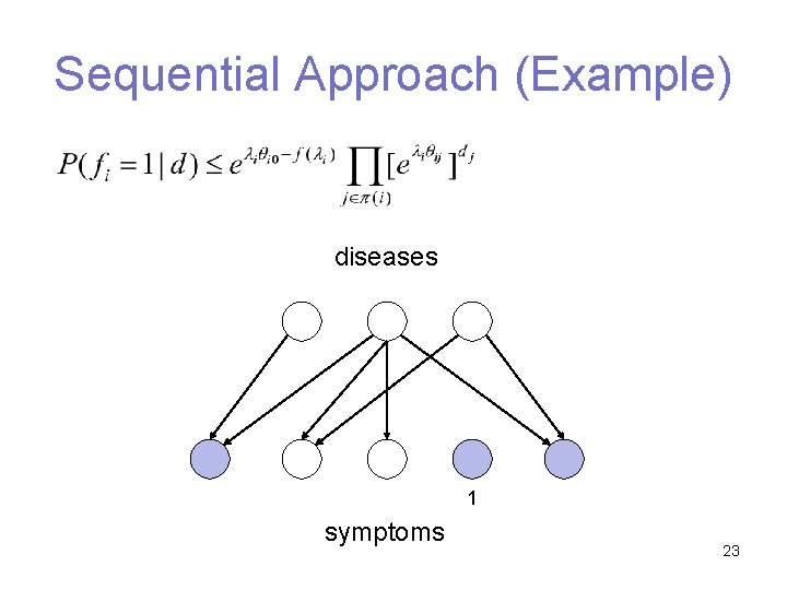
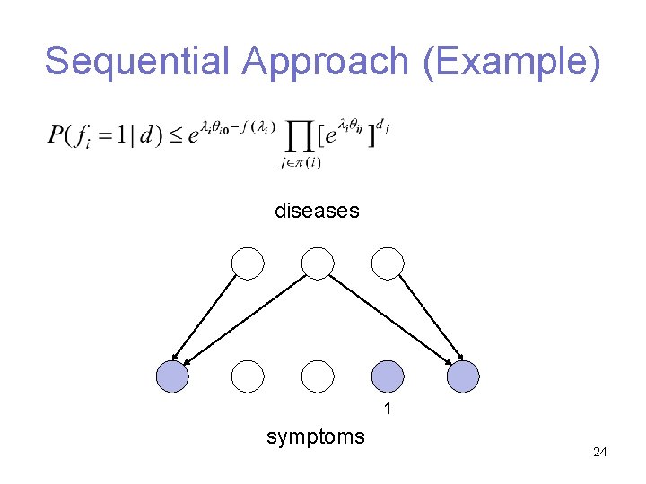
Sequential Approach (Example) diseases Log Concave symptoms 20

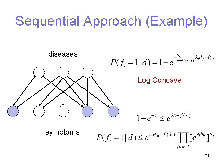
Sequential Approach (Example) diseases Log Concave symptoms 21

Sequential Approach (Example) diseases 1 symptoms 22

Sequential Approach (Example) diseases 1 symptoms 23

Sequential Approach (Example) diseases 1 symptoms 24

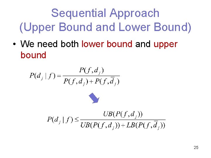
Sequential Approach (Upper Bound and Lower Bound) • We need both lower bound and upper bound 25

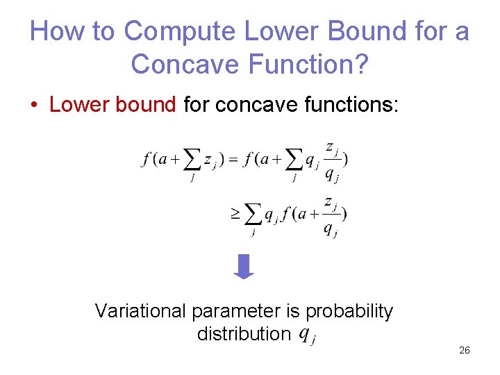
How to Compute Lower Bound for a Concave Function? • Lower bound for concave functions: Variational parameter is probability distribution 26

Block Approach (Overview) • Off-line application of sequential approach – Identify some structure amenable to exact inference – Family of probability distribution via introduction of parameters – Choose best approximation based on evidence 27

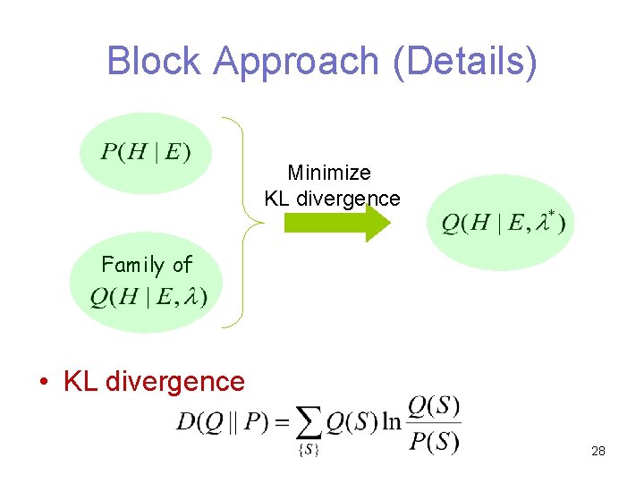
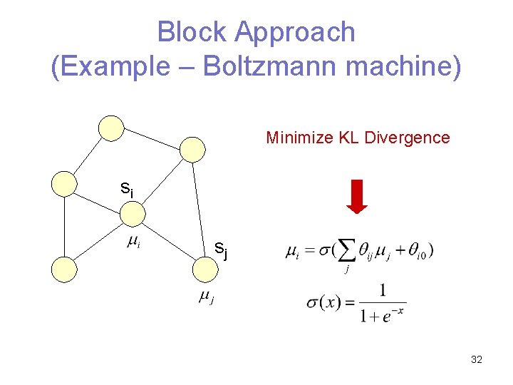
Block Approach (Details) Minimize KL divergence Family of • KL divergence 28

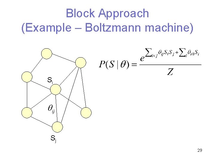
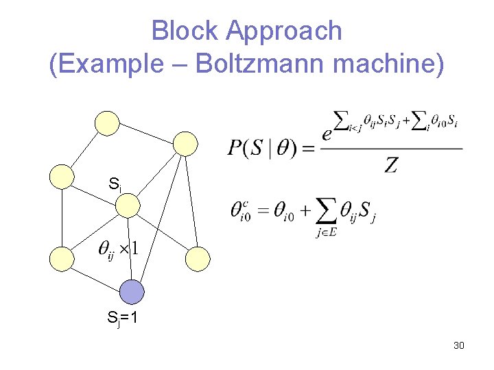
Block Approach (Example – Boltzmann machine) Si Sj 29

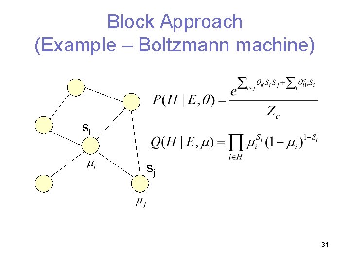
Block Approach (Example – Boltzmann machine) Si Sj=1 30

Block Approach (Example – Boltzmann machine) si sj 31

Block Approach (Example – Boltzmann machine) Minimize KL Divergence si sj 32

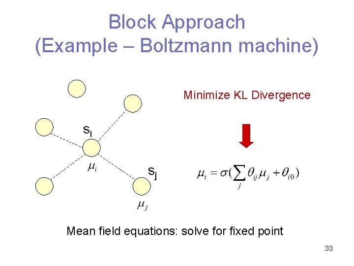
Block Approach (Example – Boltzmann machine) Minimize KL Divergence si sj Mean field equations: solve for fixed point 33

Conclusions • Time or space complexity of exact calculation is unacceptable • Complex graphs can be probabilistically simple • Inference in simplified models provides bounds on probabilities in the original model 34

35

Extra Slides 36

Concerns • • Approximation accuracy Strong dependencies can be identified Not based on convexity transformation Not able to assure that the framework will transfer to other examples • Not straightforward to develop a variational approximation for new architectures 37

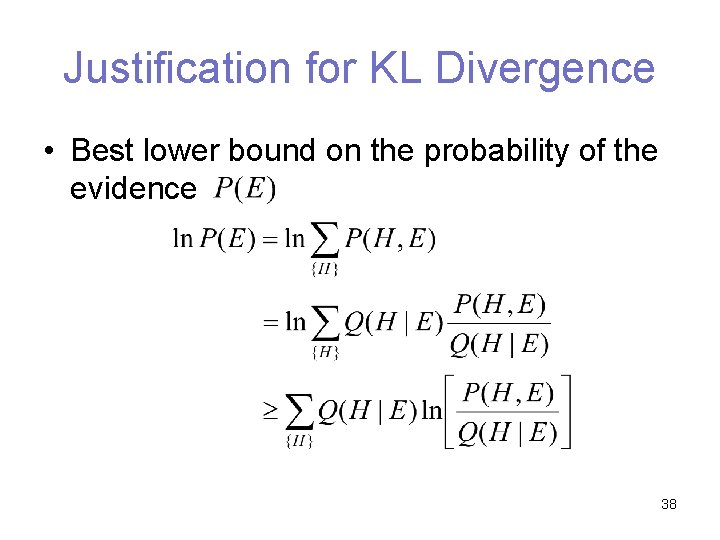
Justification for KL Divergence • Best lower bound on the probability of the evidence 38

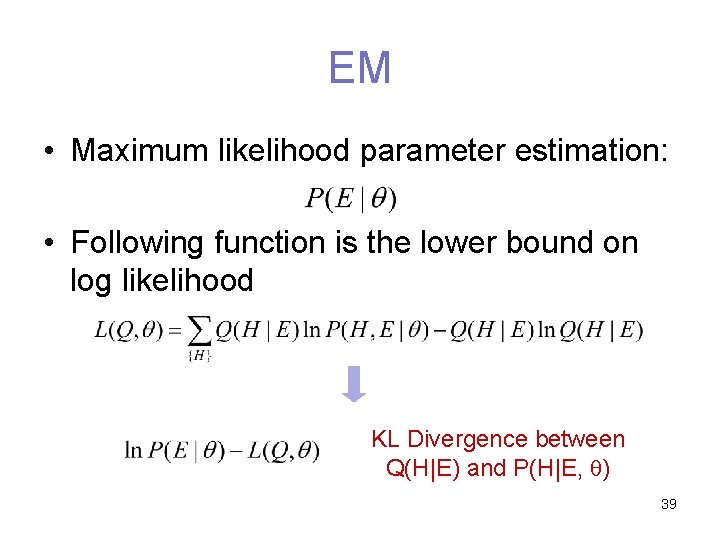
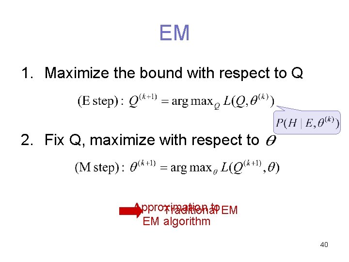
EM • Maximum likelihood parameter estimation: • Following function is the lower bound on log likelihood KL Divergence between Q(H|E) and P(H|E, ) 39

EM 1. Maximize the bound with respect to Q 2. Fix Q, maximize with respect to Approximation to EM Traditional EM algorithm 40

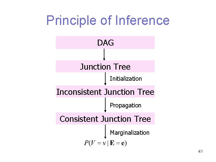
Principle of Inference DAG Junction Tree Initialization Inconsistent Junction Tree Propagation Consistent Junction Tree Marginalization 41

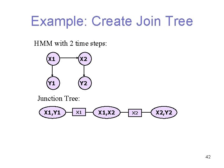
Example: Create Join Tree HMM with 2 time steps: X 1 X 2 Y 1 Y 2 Junction Tree: X 1, Y 1 X 1, X 2 X 2, Y 2 42

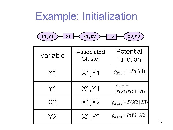
Example: Initialization X 1, Y 1 X 1, X 2 Variable Associated Cluster X 1, Y 1 X 2 X 1, X 2 Y 2 X 2, Y 2 Potential function 43

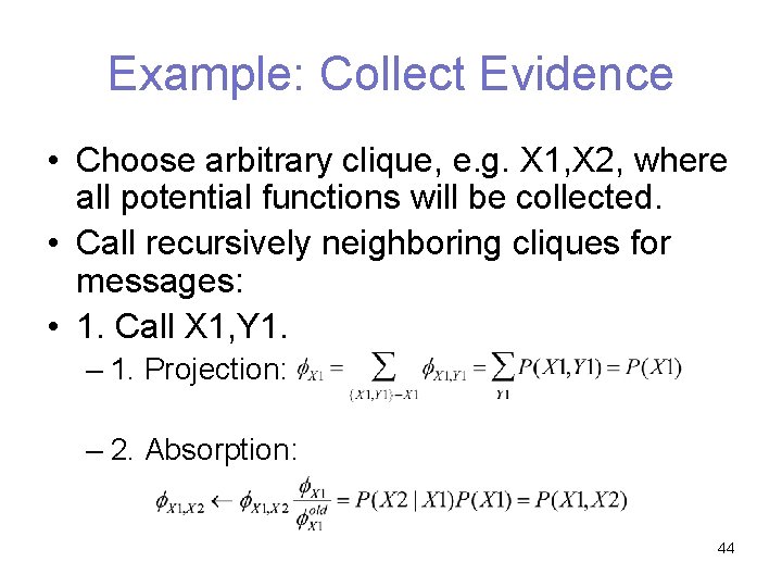
Example: Collect Evidence • Choose arbitrary clique, e. g. X 1, X 2, where all potential functions will be collected. • Call recursively neighboring cliques for messages: • 1. Call X 1, Y 1. – 1. Projection: – 2. Absorption: 44

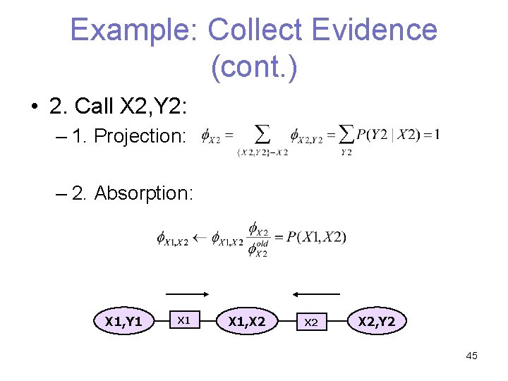
Example: Collect Evidence (cont. ) • 2. Call X 2, Y 2: – 1. Projection: – 2. Absorption: X 1, Y 1 X 1, X 2 X 2, Y 2 45

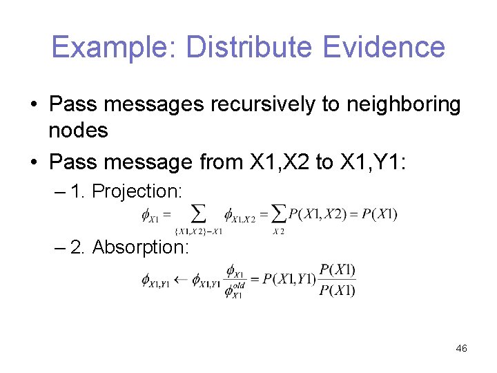
Example: Distribute Evidence • Pass messages recursively to neighboring nodes • Pass message from X 1, X 2 to X 1, Y 1: – 1. Projection: – 2. Absorption: 46

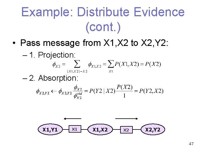
Example: Distribute Evidence (cont. ) • Pass message from X 1, X 2 to X 2, Y 2: – 1. Projection: – 2. Absorption: X 1, Y 1 X 1, X 2 X 2, Y 2 47

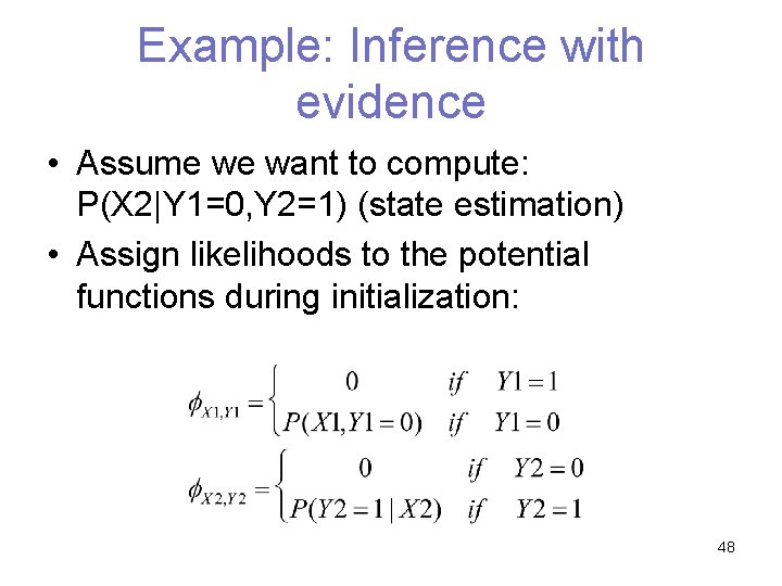
Example: Inference with evidence • Assume we want to compute: P(X 2|Y 1=0, Y 2=1) (state estimation) • Assign likelihoods to the potential functions during initialization: 48

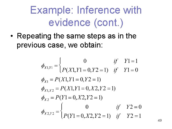
Example: Inference with evidence (cont. ) • Repeating the same steps as in the previous case, we obtain: 49

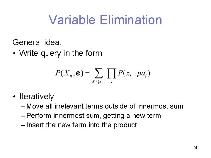
Variable Elimination General idea: • Write query in the form • Iteratively – Move all irrelevant terms outside of innermost sum – Perform innermost sum, getting a new term – Insert the new term into the product 50

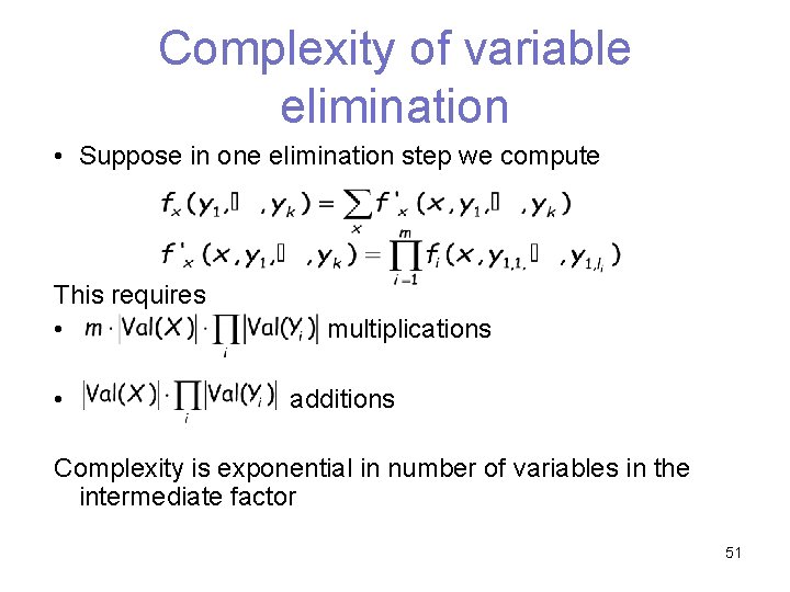
Complexity of variable elimination • Suppose in one elimination step we compute This requires • • multiplications additions Complexity is exponential in number of variables in the intermediate factor 51

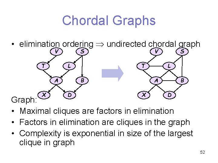
Chordal Graphs • elimination ordering undirected chordal graph S V L T X D L T B A S V B A X D Graph: • Maximal cliques are factors in elimination • Factors in elimination are cliques in the graph • Complexity is exponential in size of the largest clique in graph 52

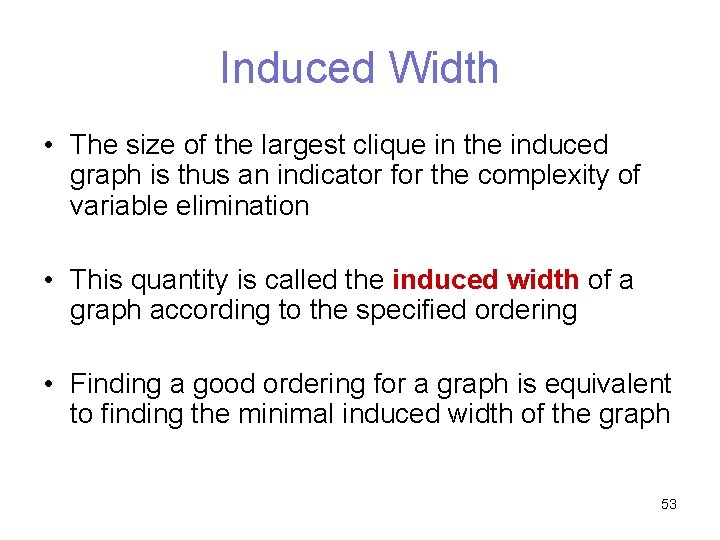
Induced Width • The size of the largest clique in the induced graph is thus an indicator for the complexity of variable elimination • This quantity is called the induced width of a graph according to the specified ordering • Finding a good ordering for a graph is equivalent to finding the minimal induced width of the graph 53

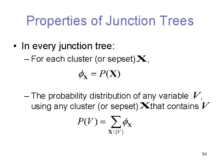
Properties of Junction Trees • In every junction tree: – For each cluster (or sepset) , – The probability distribution of any variable , using any cluster (or sepset) that contains 54

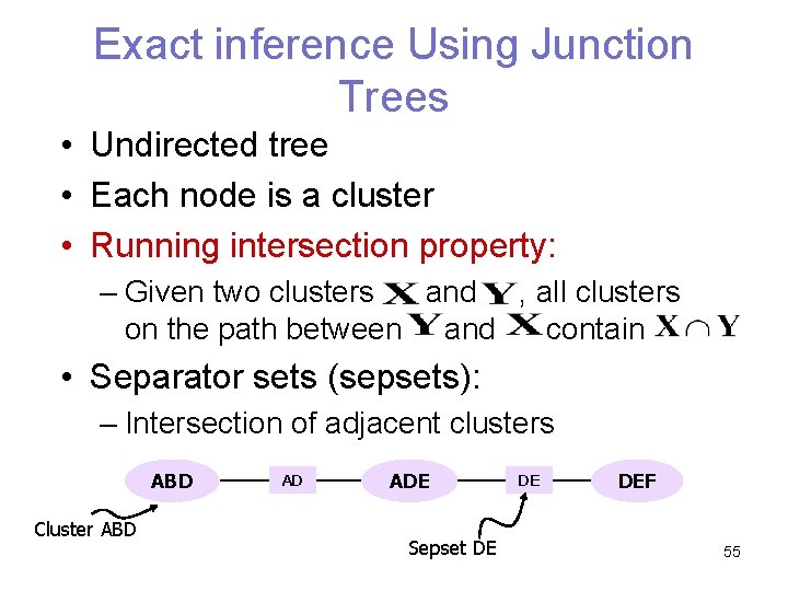
Exact inference Using Junction Trees • Undirected tree • Each node is a cluster • Running intersection property: – Given two clusters and , all clusters on the path between and contain • Separator sets (sepsets): – Intersection of adjacent clusters ABD Cluster ABD AD ADE Sepset DE DE DEF 55

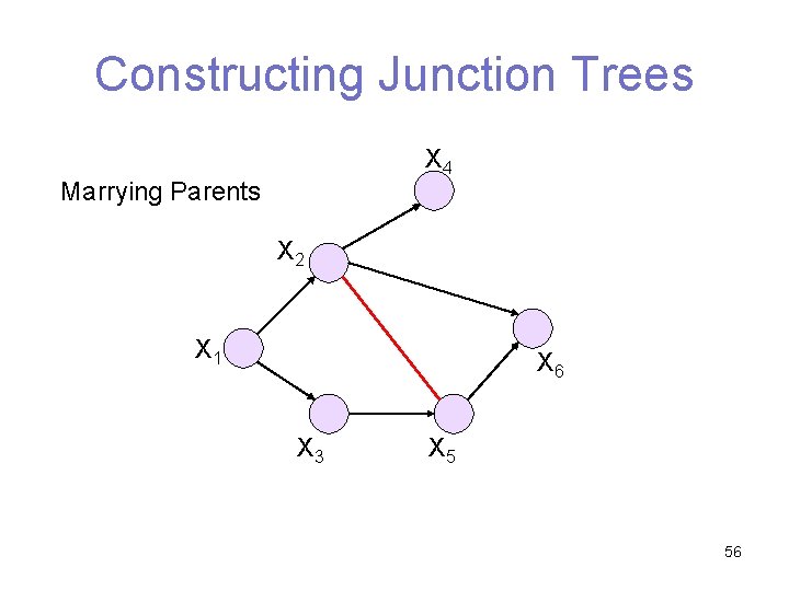
Constructing Junction Trees X 4 Marrying Parents X 2 X 1 X 6 X 3 X 5 56

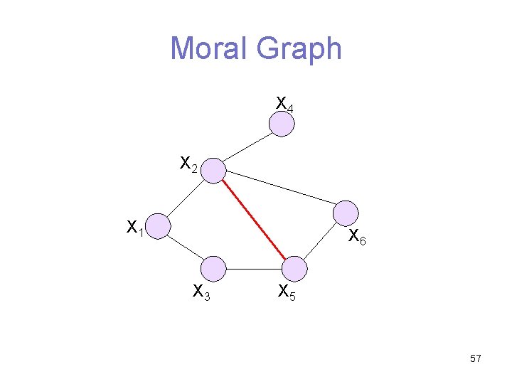
Moral Graph X 4 X 2 X 1 X 6 X 3 X 5 57

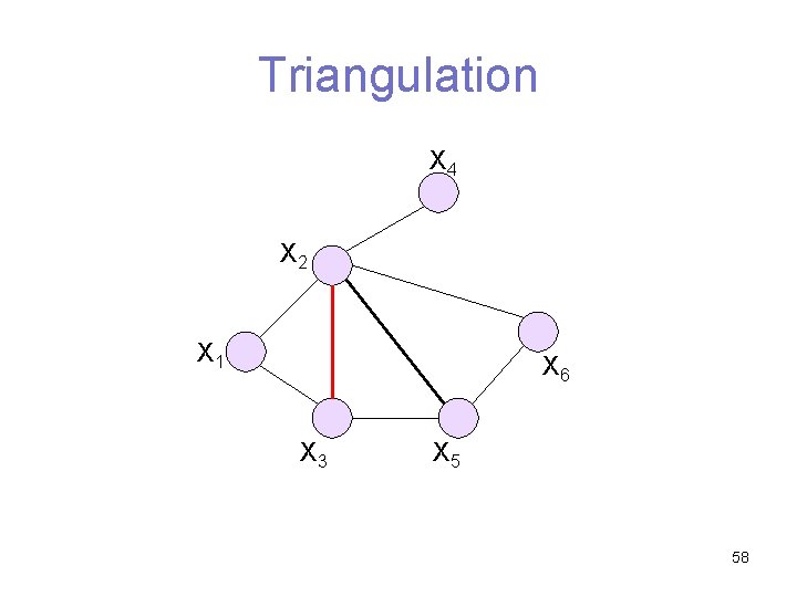
Triangulation X 4 X 2 X 1 X 6 X 3 X 5 58

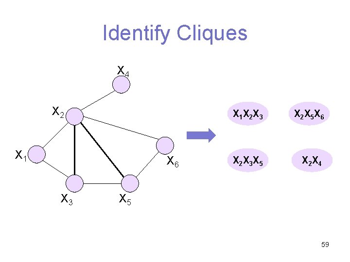
Identify Cliques X 4 X 2 X 1 X 6 X 3 X 1 X 2 X 3 X 2 X 5 X 6 X 2 X 3 X 5 X 2 X 4 X 5 59

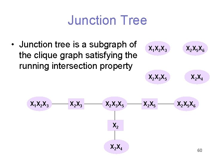
Junction Tree • Junction tree is a subgraph of the clique graph satisfying the running intersection property X 1 X 2 X 3 X 5 X 1 X 2 X 3 X 2 X 5 X 6 X 2 X 3 X 5 X 2 X 4 X 2 X 5 X 6 X 2 X 4 60

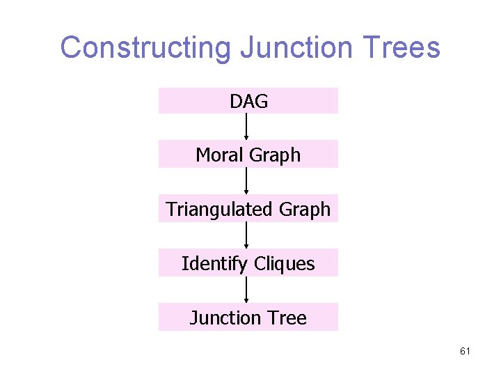
Constructing Junction Trees DAG Moral Graph Triangulated Graph Identify Cliques Junction Tree 61

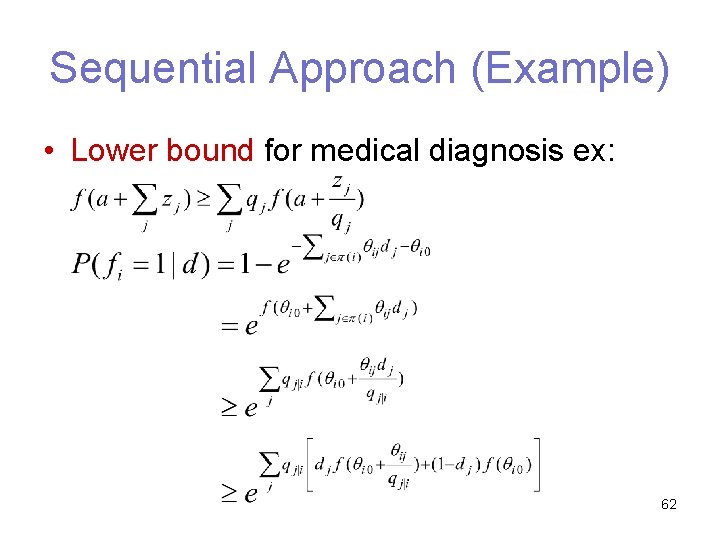
Sequential Approach (Example) • Lower bound for medical diagnosis ex: 62