Chapter 18 Decision Analysis Business Analytics Methods Models

Copyright © 2013 Pearson Education, Inc. publishing as Prentice Hall 18 -2

Chapter 18 Topics Making Decisions with Uncertain Information Decision Trees The Value of Information Utility and Decision Making Copyright © 2013 Pearson Education, Inc. publishing as Prentice Hall 18 -3

Making Decisions with Uncertain Information The purpose of business analytic models is to provide decision-makers with information needed to make decisions. There are often trade-offs to consider when making decisions. Making decisions requires human assessment of factors not included in analytic models. Understanding the philosophy of decision making and how to deal with uncertainty and risk is vitally important to being a good manager. Copyright © 2013 Pearson Education, Inc. publishing as Prentice Hall 18 -4

Making Decisions with Uncertain Information � Many decisions involve making a choice between a small set of decisions with uncertain consequences. � Such decisions involve: 1. a number of decision alternatives 2. outcomes that may occur (events) 3. payoffs associated with the events (often summarized in a payoff table) Copyright © 2013 Pearson Education, Inc. publishing as Prentice Hall 18 -5

Making Decisions with Uncertain Information Example 18. 1 Selecting a Mortgage Instrument A family is considering purchasing a new home and wants to finance $150, 000. Three mortgage options are available and the payoff table for the outcomes is shown below. The payoffs represent total interest paid under three future interest rate situations. Copyright © 2013 Pearson Education, Inc. publishing as Prentice Hall 18 -6

Making Decisions with Uncertain Information Decision Strategies for a MINIMUM Objective Average Payoff Strategy Choose the decision with the smallest average payoff. Aggressive Strategy - Minimin Choose the strategy with minimum of the smallest possible payoffs for each decision. Conservative Strategy - Minimax Choose the strategy with minimum of the largest possible payoffs for each decision. Opportunity Loss Strategy - Minimax Regret Choose the strategy with the minimum opportunityloss: its payoff – best payoff for that outcome Copyright © 2013 Pearson Education, Inc. publishing as Prentice Hall 18 -7

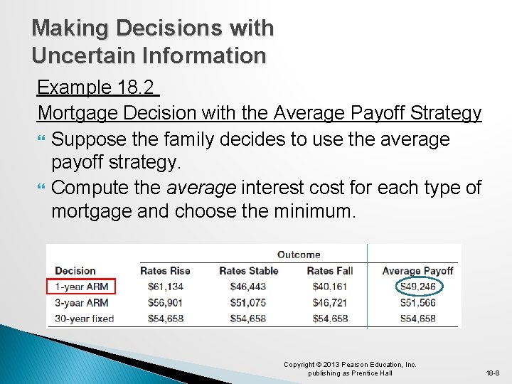
Making Decisions with Uncertain Information Example 18. 2 Mortgage Decision with the Average Payoff Strategy Suppose the family decides to use the average payoff strategy. Compute the average interest cost for each type of mortgage and choose the minimum. Copyright © 2013 Pearson Education, Inc. publishing as Prentice Hall 18 -8

Making Decisions with Uncertain Information Example 18. 3 Mortgage Decision with the Aggressive Strategy Suppose the family decides to use the aggressive minimin payoff strategy. Determine the lowest interest cost for each type of mortgage and choose the minimum. Copyright © 2013 Pearson Education, Inc. publishing as Prentice Hall 18 -9

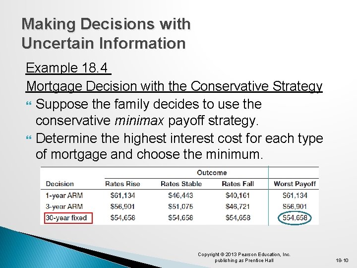
Making Decisions with Uncertain Information Example 18. 4 Mortgage Decision with the Conservative Strategy Suppose the family decides to use the conservative minimax payoff strategy. Determine the highest interest cost for each type of mortgage and choose the minimum. Copyright © 2013 Pearson Education, Inc. publishing as Prentice Hall 18 -10

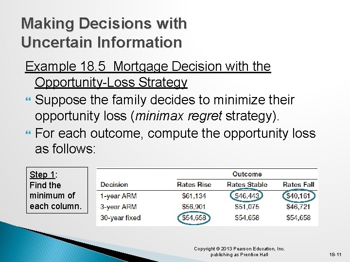
Making Decisions with Uncertain Information Example 18. 5 Mortgage Decision with the Opportunity-Loss Strategy Suppose the family decides to minimize their opportunity loss (minimax regret strategy). For each outcome, compute the opportunity loss as follows: Step 1: Find the minimum of each column. Copyright © 2013 Pearson Education, Inc. publishing as Prentice Hall 18 -11

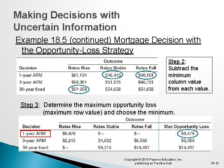
Making Decisions with Uncertain Information Example 18. 5 (continued) Mortgage Decision with the Opportunity-Loss Strategy a Step 2: Subtract the minimum column value from each value. Step 3: Determine the maximum opportunity loss (maximum row value) and choose the minimum. Copyright © 2013 Pearson Education, Inc. publishing as Prentice Hall 18 -12

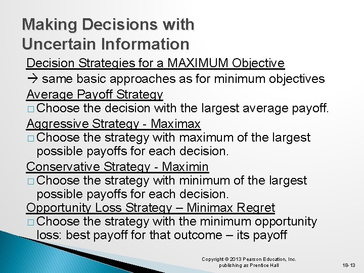
Making Decisions with Uncertain Information Decision Strategies for a MAXIMUM Objective same basic approaches as for minimum objectives Average Payoff Strategy � Choose the decision with the largest average payoff. Aggressive Strategy - Maximax � Choose the strategy with maximum of the largest possible payoffs for each decision. Conservative Strategy - Maximin � Choose the strategy with minimum of the largest possible payoffs for each decision. Opportunity Loss Strategy – Minimax Regret � Choose the strategy with the minimum opportunity loss: best payoff for that outcome – its payoff Copyright © 2013 Pearson Education, Inc. publishing as Prentice Hall 18 -13

Making Decisions with Uncertain Information Example 18. 6 Evaluating Risk in the Mortgage Decision � Suppose the family has obtained the standard deviations of the interest costs associated with each loan type. � While none of the previous payoff strategies chose the 3 -year ARM, it may be attractive to the family due to its moderate risk level and potential upside at stable and falling interest rates. Copyright © 2013 Pearson Education, Inc. publishing as Prentice Hall 18 -14

Making Decisions with Uncertain Information Example 18. 7 Mortgage Decision with the Expected Value Strategy � Suppose the family has obtained probability information concerning future interest rates. � For each loan type, compute the expected value of the interest cost and choose the minimum. Copyright © 2013 Pearson Education, Inc. publishing as Prentice Hall 18 -15

Making Decisions with Uncertain Information Summary of Decision Strategies Under Uncertainty Table 18. 1

Decision Trees Decision trees, which consist of nodes and branches, are a useful approach to structuring decision problems involving uncertainty. Nodes are points in time at which events take place. Decision nodes are nodes in which a decision takes place by choosing among several alternatives (typically denoted as squares). Event nodes are nodes in which an event occurs not controlled by the decision-maker (typically denoted as circles). Copyright © 2013 Pearson Education, Inc. publishing as Prentice Hall 18 -17

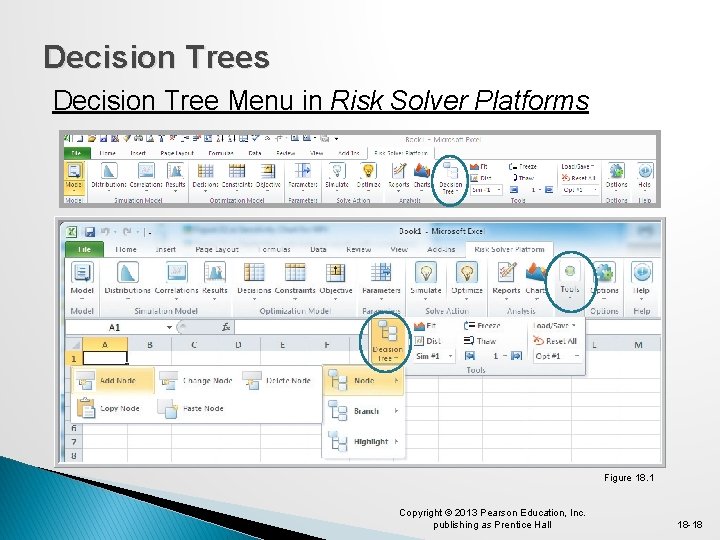
Decision Trees Decision Tree Menu in Risk Solver Platforms Figure 18. 1 Copyright ©

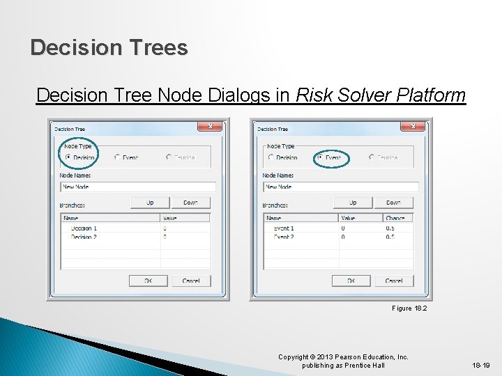
Decision Trees Decision Tree Node Dialogs in Risk Solver Platform Figure 18. 2 Copyright

Decision Trees Example 18. 8 Creating a Decision Tree For the mortgage selection problem, create a decision tree using Risk Solver. To start the decision tree, add a node for selection of the loan type. Then, for each type of loan, add a node for selection of the uncertain interest rate conditions. Copyright © 2013 Pearson Education, Inc. publishing as Prentice Hall 18 -20

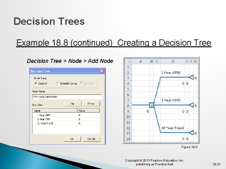
Decision Trees Example 18. 8 (continued) Creating a Decision Tree > Node > Add

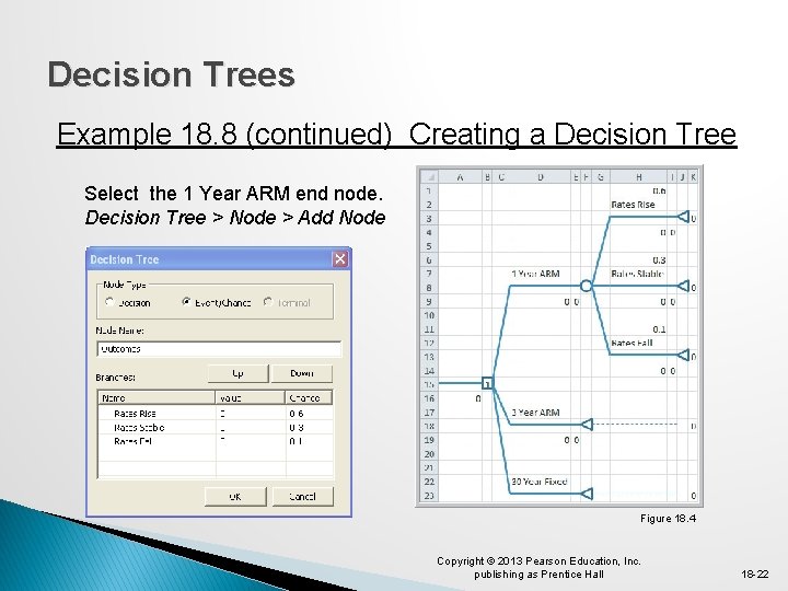
Decision Trees Example 18. 8 (continued) Creating a Decision Tree Select the 1 Year ARM end node. Decision Tree > Node > Add Node Figure 18. 4 Copyright © 2013 Pearson Education, Inc. publishing as Prentice Hall 18 -22

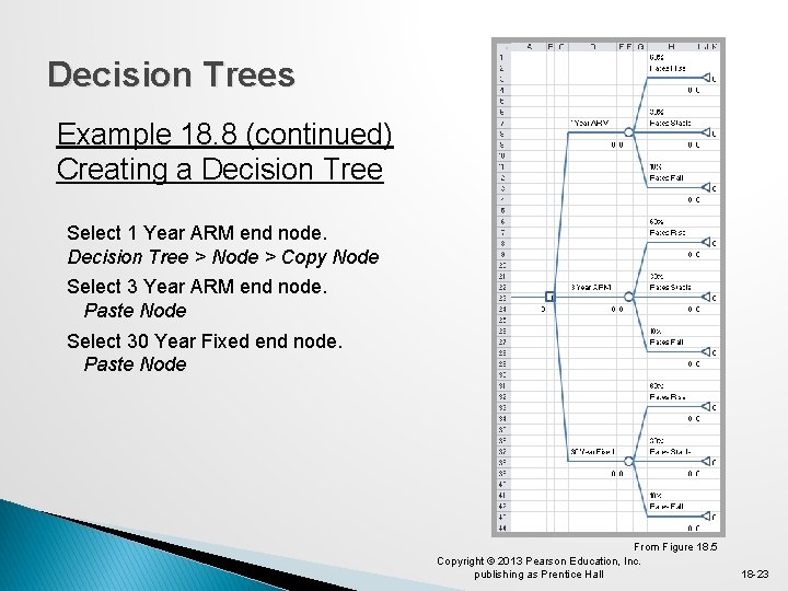
Decision Trees Example 18. 8 (continued) Creating a Decision Tree Select 1 Year ARM end node. Decision Tree > Node > Copy Node Select 3 Year ARM end node. Paste Node Select 30 Year Fixed end node. Paste Node From Figure 18. 5 Copyright © 2013 Pearson Education, Inc. publishing as Prentice Hall 18 -23

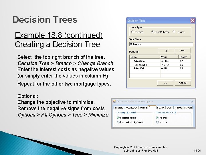
Decision Trees Example 18. 8 (continued) Creating a Decision Tree Select the top right branch of the tree. Decision Tree > Branch > Change Branch Enter the interest costs as negative values (or simply enter the values in column H). Repeat for the other two mortgage types. Optional: Change the objective to minimize. Remove the negative signs from costs. Options > All Options > Tree > Minimize Copyright © 2013 Pearson Education, Inc. publishing as Prentice Hall 18 -24

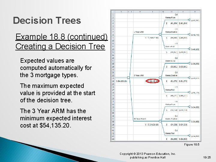
Decision Trees Example 18. 8 (continued) Creating a Decision Tree Expected values are computed automatically for the 3 mortgage types. The maximum expected value is provided at the start of the decision tree. The 3 Year ARM has the minimum expected interest cost at $54, 135. 20. Figure 18. 5 Copyright © 2013 Pearson Education, Inc. publishing as Prentice Hall 18 -25

Decision Trees Example 18. 8 (continued) Creating a Decision Tree Solved as a Minimization Problem Best decision can be highlighted Decision Tree Highlight Best From Figure 18. 5 Copyright © 2013 Pearson Education, Inc. publishing as Prentice Hall 18 -26

Decision Trees Example 18. 8 (continued) Creating a Decision Tree Viewing Solver’s Excel Formulas

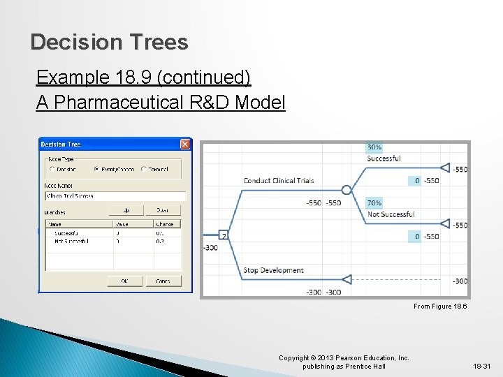
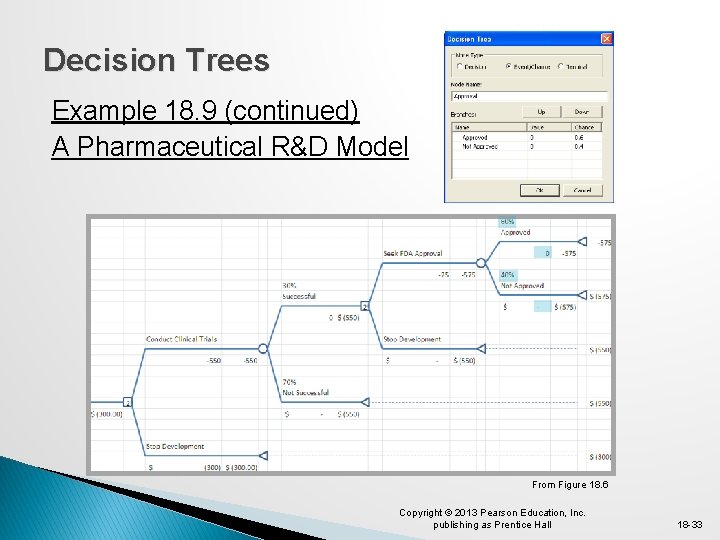
Decision Trees Example 18. 9 A Pharmaceutical R&D Model Moore Pharmaceuticals (Example 8. 3) needs to decide whether to conduct clinical trials and seek FDA approval for a newly developed drug. $300 million has already been spent on research. The next decision is whether to conduct clinical trials at a cost of $250 million. 30% is the likelihood of success following trials. If the trials are successful, the next decision is whether to seek FDA approval, costing $25 million. 60% is likelihood of FDA approval. Copyright © 2013 Pearson Education, Inc. publishing as Prentice Hall 18 -28

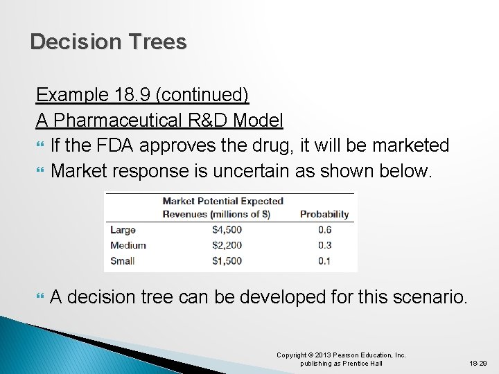
Decision Trees Example 18. 9 (continued) A Pharmaceutical R&D Model If the FDA approves the drug, it will be marketed Market response is uncertain as shown below. A decision tree can be developed for this scenario. Copyright © 2013 Pearson Education, Inc. publishing as Prentice Hall 18 -29

Decision Trees Example 18. 9 (continued) A Pharmaceutical R&D Model From Figure 18. 6

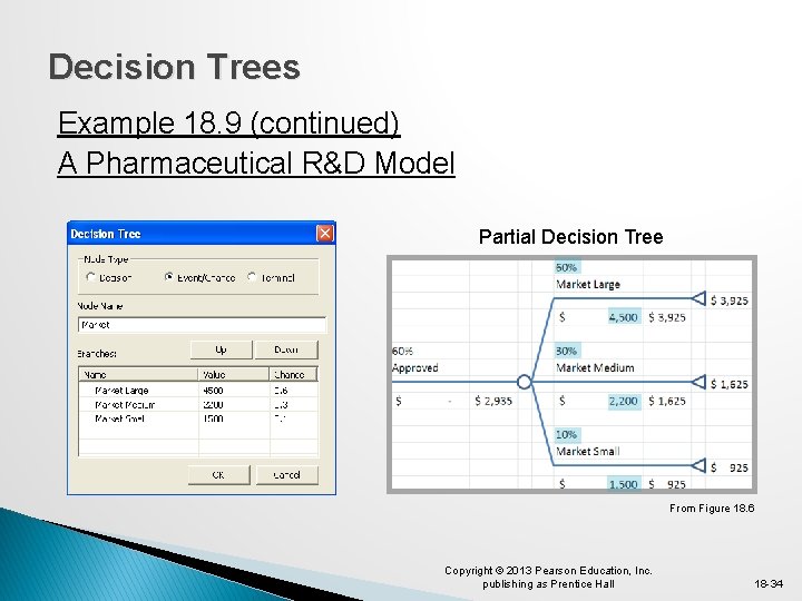
Decision Trees Example 18. 9 (continued) A Pharmaceutical R&D Model Partial Decision Tree From

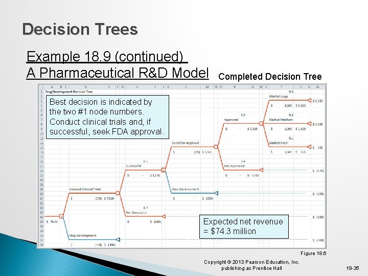
Decision Trees Example 18. 9 (continued) A Pharmaceutical R&D Model Completed Decision Tree Best decision is indicated by the two #1 node numbers. Conduct clinical trials and, if successful, seek FDA approval. Expected net revenue = $74. 3 million Figure 18. 6 Copyright © 2013 Pearson Education, Inc. publishing as Prentice Hall 18 -35

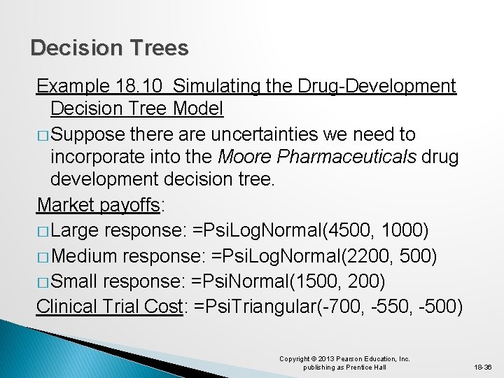
Decision Trees Example 18. 10 Simulating the Drug-Development Decision Tree Model � Suppose there are uncertainties we need to incorporate into the Moore Pharmaceuticals drug development decision tree. Market payoffs: � Large response: =Psi. Log. Normal(4500, 1000) � Medium response: =Psi. Log. Normal(2200, 500) � Small response: =Psi. Normal(1500, 200) Clinical Trial Cost: =Psi. Triangular(-700, -550, -500) Copyright © 2013 Pearson Education, Inc. publishing as Prentice Hall 18 -36

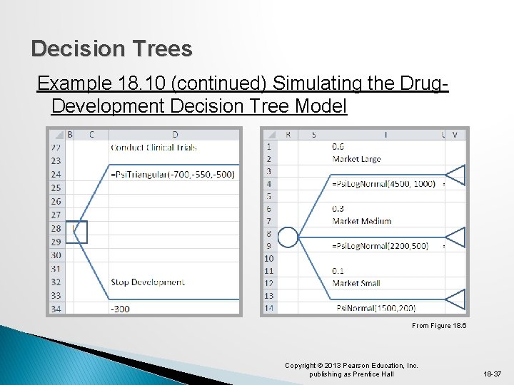
Decision Trees Example 18. 10 (continued) Simulating the Drug. Development Decision Tree Model From

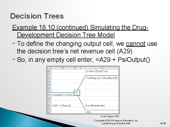
Decision Trees Example 18. 10 (continued) Simulating the Drug. Development Decision Tree Model To define the changing output cell, we cannot use the decision tree’s net revenue cell (A 29). So, in any empty cell enter, =A 29 + Psi. Output() From Figure 18. 6 Copyright © 2013 Pearson Education, Inc. publishing as Prentice Hall 18 -38

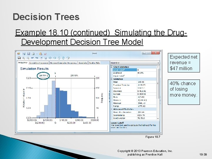
Decision Trees Example 18. 10 (continued) Simulating the Drug. Development Decision Tree Model Expected net revenue = $47 million 40% chance of losing more money. Figure 18. 7 Copyright © 2013 Pearson Education, Inc. publishing as Prentice Hall 18 -39

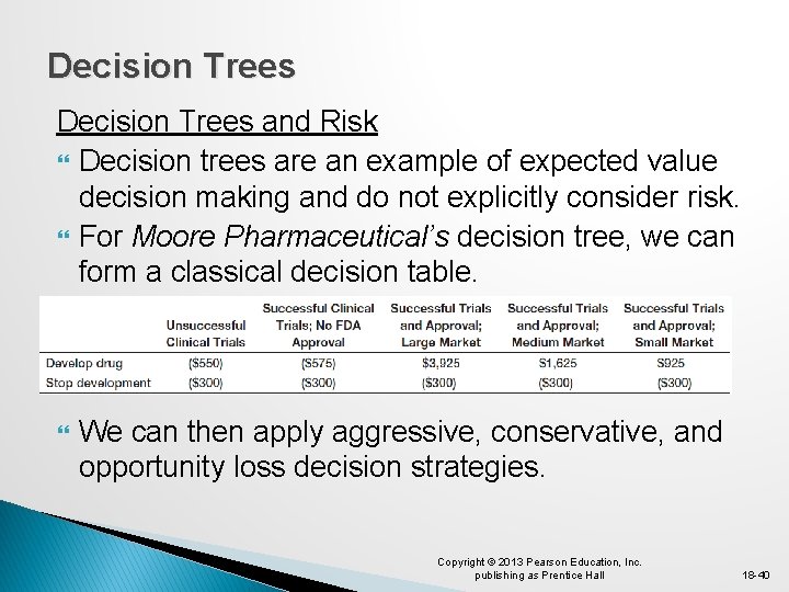
Decision Trees and Risk Decision trees are an example of expected value decision making and do not explicitly consider risk. For Moore Pharmaceutical’s decision tree, we can form a classical decision table. We can then apply aggressive, conservative, and opportunity loss decision strategies. Copyright © 2013 Pearson Education, Inc. publishing as Prentice Hall 18 -40

Decision Trees and Risk (continued) Copyright © 2013 Pearson Education, Inc. publishing as Prentice

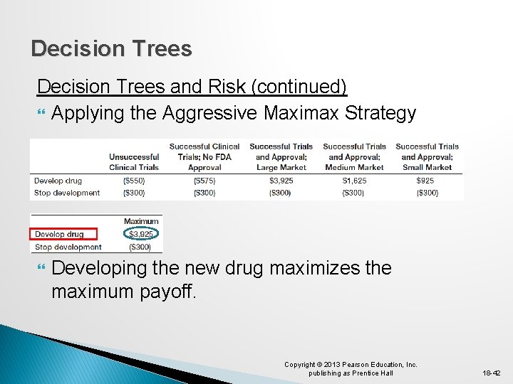
Decision Trees and Risk (continued) Applying the Aggressive Maximax Strategy Developing the new drug maximizes the maximum payoff. Copyright © 2013 Pearson Education, Inc. publishing as Prentice Hall 18 -42

Decision Trees and Risk (continued) Applying the Conservative Maximin Strategy Stopping development of the new drug maximizes the minimum payoff. Copyright © 2013 Pearson Education, Inc. publishing as Prentice Hall 18 -43

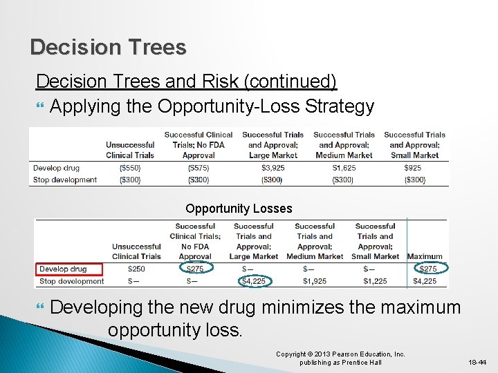
Decision Trees and Risk (continued) Applying the Opportunity-Loss Strategy Opportunity Losses Developing the new drug minimizes the maximum opportunity loss. Copyright © 2013 Pearson Education, Inc. publishing as Prentice Hall 18 -44

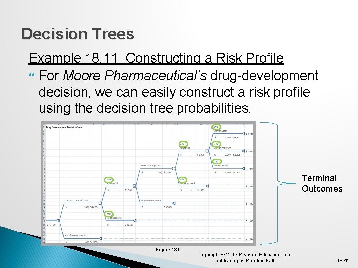
Decision Trees Example 18. 11 Constructing a Risk Profile For Moore Pharmaceutical’s drug-development decision, we can easily construct a risk profile using the decision tree probabilities. Terminal Outcomes Figure 18. 6 Copyright © 2013 Pearson Education, Inc. publishing as Prentice Hall 18 -45

Decision Trees Example 18. 11 (continued) Constructing a Risk Profile Compute the probability of each terminal outcome. P(Large market) = (. 3)(. 6) = 0. 108 P(Medium market) = (. 3)(. 6)(. 3) = 0. 054 P(Small market) = (. 3)(. 6)(. 1) = 0. 018 P(FDA not approved) = (. 3)(. 4) = 0. 120 P(Clinical trials not successful) = 0. 700 SUM 1. 000 Copyright © 2013 Pearson Education, Inc. publishing as Prentice Hall 18 -46

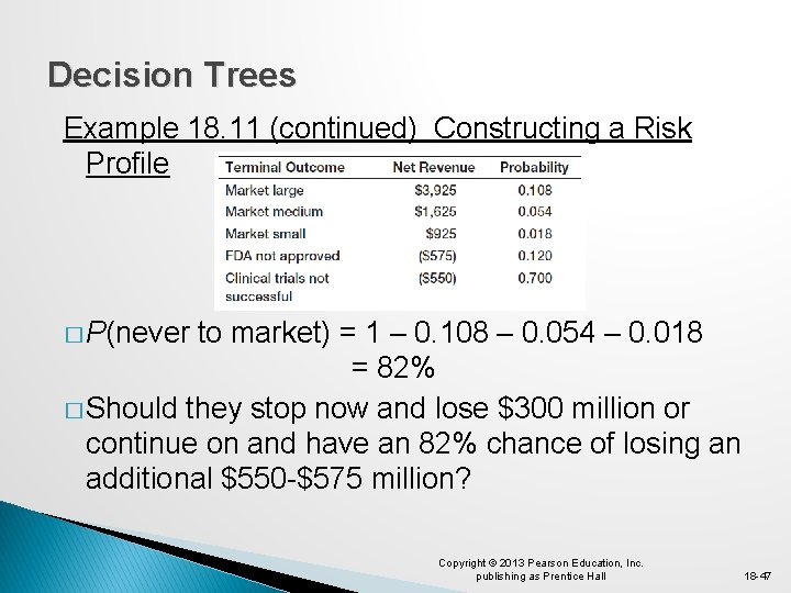
Decision Trees Example 18. 11 (continued) Constructing a Risk Profile � P(never to market) = 1 – 0. 108 – 0. 054 – 0. 018 = 82% � Should they stop now and lose $300 million or continue on and have an 82% chance of losing an additional $550 -$575 million? Copyright © 2013 Pearson Education, Inc. publishing as Prentice Hall 18 -47

Decision Trees Example 18. 12 Sensitivity Analysis for Airline Revenue Management Decisions Recall Example 5. 21 - Airline Revenue Management � Full and discount airfares are available for a flight. � Full-fare ticket costs $560 � Discount ticket costs $400 � X = selling price of a ticket � p = 0. 75 (the probability of selling a full-fare ticket) � E[X] = 0. 75($560) + 0. 25(0) = $420 � Breakeven point: $400 = p($560) or p = 0. 714 Copyright © 2013 Pearson Education, Inc. publishing as Prentice Hall 18 -48

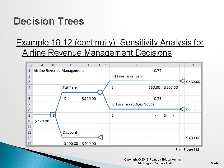
Decision Trees Example 18. 12 (continuity) Sensitivity Analysis for Airline Revenue Management Decisions From

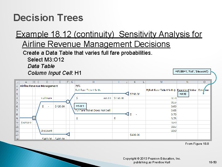
Decision Trees Example 18. 12 (continuity) Sensitivity Analysis for Airline Revenue Management Decisions Create a Data Table that varies full fare probabilities. Select M 3: O 12 Data Table Column Input Cell: H 1 =IF(B 9=1, ”Full”, ”Discount”) =A 10 =1 -H 1 From Figure 18. 8 Copyright © 2013 Pearson Education, Inc. publishing as Prentice Hall 18 -50

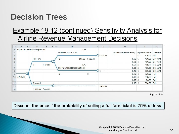
Decision Trees Example 18. 12 (continued) Sensitivity Analysis for Airline Revenue Management Decisions Figure 18. 8 Discount the price if the probability of selling a full fare ticket is 70% or less. Copyright © 2013 Pearson Education, Inc. publishing as Prentice Hall 18 -51

The Value of Information Expected Value of Perfect Information (EVPI) � The value of information is the improvement in return if additional information is acquired. � Perfect information tell us, with certainty, which outcome will occur. � EVPI is expected monetary value (EMV) with perfect information minus the EMV without it. � Expected opportunity loss is the average additional amount the investor would have achieved if the correct decision had been made. � Minimizing expected opportunity loss always results in the same decision as maximizing expected value. Copyright © 2013 Pearson Education, Inc. publishing as Prentice Hall 18 -52

The Value of Information Example 18. 13 Finding EVPI for the Mortgage-Selection Decision Opportunity

The Value of Information Example 18. 13 (continued) Finding EVPI for the Mortgage-Selection Decision Best decision $54, 658 Difference = EVPI $46, 443 $40, 161 $50. 743. 80 $3391. 40 The family should not pay more than $3391. 40 for any information about future interest rates, no matter how good. Copyright © 2013 Pearson Education, Inc. publishing as Prentice Hall 18 -54

The Value of Information Decisions with Sample Information � Sample information is the result of conducting some type of experiment. � Examples include marketing research studies or interviewing experts. � Sample information is always imperfect and often comes at a cost. � The expected value of sample information (EVSI) is the EMV of the outcome with sample information minus the EMV without it. Copyright © 2013 Pearson Education, Inc. publishing as Prentice Hall 18 -55

The Value of Information Example 18. 14 Decisions with Sample Information � A company is developing a new cell phone and currently has two models under consideration. � 70% of their new phones have high consumer demand 30% have low consumer demand. � Model 1 requires $200, 000 investment. If demand is high, revenue = $500, 000 If demand is low, revenue = $160, 000 � Model 2 requires $175, 000 investment. If demand is high, revenue = $450, 000 If demand is low, revenue = $160, 000 Copyright © 2013 Pearson Education, Inc. publishing as Prentice Hall 18 -56

The Value of Information Example 18. 14 (continued) Decisions with Sample Information Decision tree units are $000. Choose Model 1 Expected profit = $198, 000 Figure 18. 9 Copyright © 2013 Pearson Education, Inc. publishing as Prentice Hall 18 -57

The Value of Information Example 18. 14 (continued) Decisions with Sample Information Suppose a market research study is conducted. It is known that market research is not completely accurate since, in the past: 90% of all products that had high consumer demand received high market survey responses. 20% of all products that had low consumer demand received high market survey responses. We can update the decision tree using Bayes’s rule. Copyright © 2013 Pearson Education, Inc. publishing as Prentice Hall 18 -58

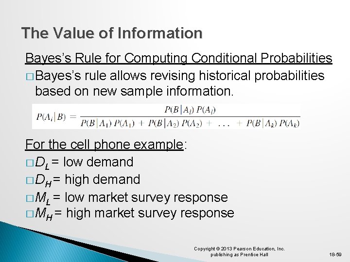
The Value of Information Bayes’s Rule for Computing Conditional Probabilities � Bayes’s rule allows revising historical probabilities based on new sample information. For the cell phone example: � DL = low demand � DH = high demand � ML = low market survey response � MH = high market survey response Copyright © 2013 Pearson Education, Inc. publishing as Prentice Hall 18 -59

The Value of Information Example 18. 15 Applying Bayes’s Rule to Compute Conditional Probabilities P(DH) = 0. 70 P(DL) = 0. 30 P(MH |DH) = 0. 90 P(ML |DH) = 1 − 0. 90 = 0. 10 P(MH |DL) = 0. 20 P(ML |DL) = 1 − 0. 20 = 0. 80 P(DH |MH) = (. 9)(. 7)/[(. 9)(. 7)+(. 2)(. 3)] = 0. 913 P(DL |MH) = 1 − 0. 913 = 0. 087 P(DH |ML) = (. 1)(. 7)/[(. 1)(. 7)+(. 8)(. 3)] = 0. 226 P(DL |ML) = 1 − 0. 226 = 0. 774 Copyright © 2013 Pearson Education, Inc. publishing as Prentice Hall 18 -60

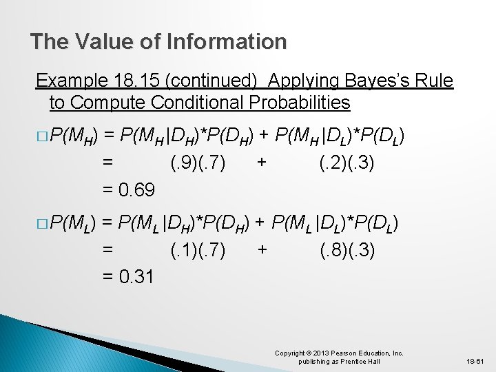
The Value of Information Example 18. 15 (continued) Applying Bayes’s Rule to Compute Conditional Probabilities � P(MH) = P(MH |DH)*P(DH) + P(MH |DL)*P(DL) = (. 9)(. 7) + (. 2)(. 3) = 0. 69 � P(ML) = P(ML |DH)*P(DH) + P(ML |DL)*P(DL) = (. 1)(. 7) + (. 8)(. 3) = 0. 31 Copyright © 2013 Pearson Education, Inc. publishing as Prentice Hall 18 -61

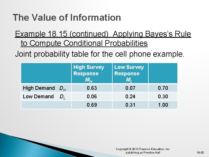
The Value of Information Example 18. 15 (continued) Applying Bayes’s Rule to Compute Conditional Probabilities Joint probability table for the cell phone example. High Survey Response MH Low Survey Response ML High Demand DH 0. 63 0. 07 0. 70 Low Demand 0. 06 0. 24 0. 30 0. 69 0. 31 1. 00 DL Copyright © 2013 Pearson Education, Inc. publishing as Prentice Hall 18 -62

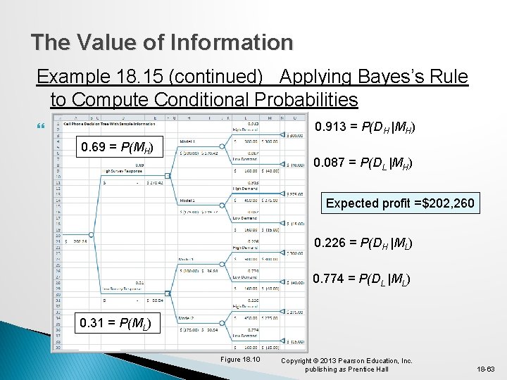
The Value of Information Example 18. 15 (continued) Applying Bayes’s Rule to Compute Conditional Probabilities 0. 913 = P(DH |MH) 0. 69 = P(MH) 0. 087 = P(DL |MH) Expected profit =$202, 260 0. 226 = P(DH |ML) 0. 774 = P(DL |ML) 0. 31 = P(ML) Figure 18. 10 Copyright © 2013 Pearson Education, Inc. publishing as Prentice Hall 18 -63

The Value of Information Example 18. 15 (continued) Applying Bayes’s Rule to Compute Conditional Probabilities The expected profit in Example 18. 14 (without additional information) is $198, 000. The expected profit in Example 18. 15 (with additional information) is $202, 260. The EVSI = $4260. The company should not pay more than $4260 for a market research survey. Figure 18. 10 Copyright © 2013 Pearson Education, Inc. publishing as Prentice Hall 18 -64

Utility and Decision Making � Utility theory is an approach for assessing risk attitudes quantitatively. � An individual’s utility function reflects their preference toward risk. � The risk premium is the payoff amount that an individual is willing to forgo to avoid risk. � The break-even probability is the point at which an individual is indifferent between a guaranteed payoff and taking a gamble for a higher payoff. � The certainty equivalent is the amount an individual feels is equivalent to the payoff from an uncertain gamble. Copyright © 2013 Pearson Education, Inc. publishing as Prentice Hall 18 -65

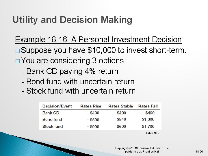
Utility and Decision Making Example 18. 16 A Personal Investment Decision � Suppose you have $10, 000 to invest short-term. � You are considering 3 options: - Bank CD paying 4% return - Bond fund with uncertain return - Stock fund with uncertain return Table 18. 2 Copyright © 2013 Pearson Education, Inc. publishing as Prentice Hall 18 -66

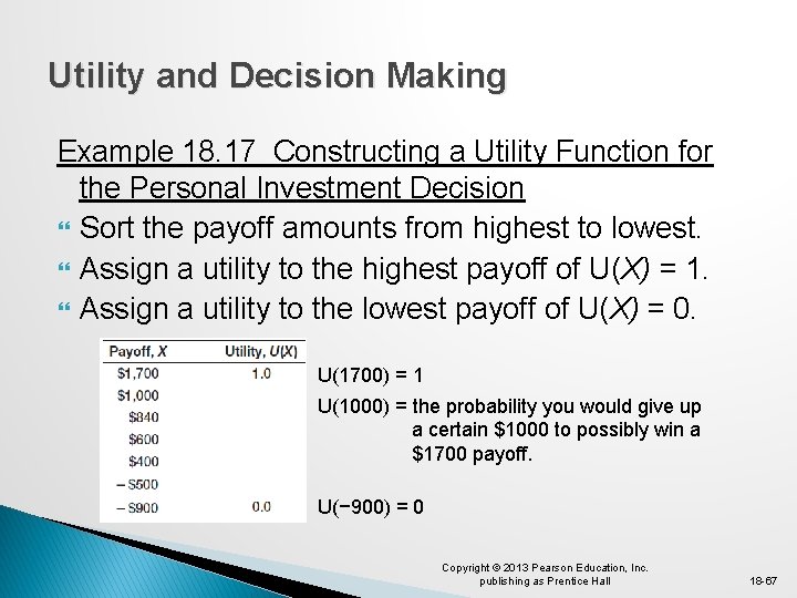
Utility and Decision Making Example 18. 17 Constructing a Utility Function for the Personal Investment Decision Sort the payoff amounts from highest to lowest. Assign a utility to the highest payoff of U(X) = 1. Assign a utility to the lowest payoff of U(X) = 0. U(1700) = 1 U(1000) = the probability you would give up a certain $1000 to possibly win a $1700 payoff. U(− 900) = 0 Copyright © 2013 Pearson Education, Inc. publishing as Prentice Hall 18 -67

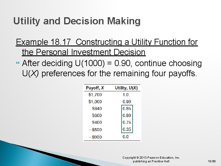
Utility and Decision Making Example 18. 17 Constructing a Utility Function for the Personal Investment Decision After deciding U(1000) = 0. 90, continue choosing U(X) preferences for the remaining four payoffs. Copyright © 2013 Pearson Education, Inc. publishing as Prentice Hall 18 -68

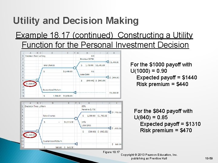
Utility and Decision Making Example 18. 17 (continued) Constructing a Utility Function for the Personal Investment Decision For the $1000 payoff with U(1000) = 0. 90 Expected payoff = $1440 Risk premium = $440 For the $840 payoff with U(840) = 0. 85 Expected payoff = $1310 Risk premium = $470 Figure 18. 17 Copyright © 2013 Pearson Education, Inc. publishing as Prentice Hall 18 -69

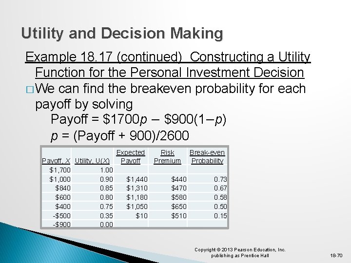
Utility and Decision Making Example 18. 17 (continued) Constructing a Utility Function for the Personal Investment Decision � We can find the breakeven probability for each payoff by solving Payoff = $1700 p − $900(1−p) p = (Payoff + 900)/2600 Payoff, X Utility, U(X) $1, 700 1. 00 $1, 000 0. 90 $840 0. 85 $600 0. 80 $400 0. 75 -$500 0. 35 -$900 0. 00 Expected Payoff $1, 440 $1, 310 $1, 180 $1, 050 $10 Risk Premium $440 $470 $580 $650 $510 Break-even Probability 0. 73 0. 67 0. 58 0. 50 0. 15 Copyright © 2013 Pearson Education, Inc. publishing as Prentice Hall 18 -70

Utility and Decision Making Example 18. 17 (continued) Constructing a Utility Function for the Personal Investment Decision Risk Aversion Risk premiums > 0 U(X) > Risk neutral Concave downward Figure 18. 12 Copyright © 2013 Pearson Education, Inc. publishing as Prentice Hall 18 -71

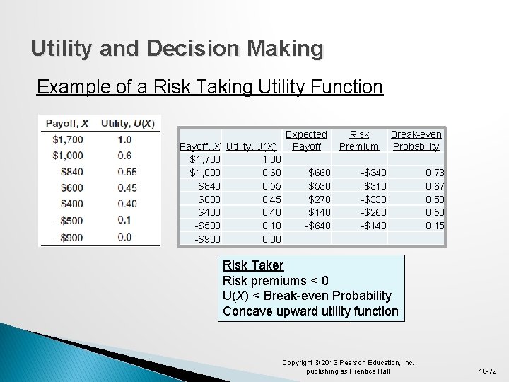
Utility and Decision Making Example of a Risk Taking Utility Function Payoff, X $1, 700 $1, 000 $840 $600 $400 -$500 -$900 Expected Risk Break-even Utility, U(X) Payoff Premium Probability 1. 00 0. 60 $660 -$340 0. 73 0. 55 $530 -$310 0. 67 0. 45 $270 -$330 0. 58 0. 40 $140 -$260 0. 50 0. 10 -$640 -$140 0. 15 0. 00 Risk Taker Risk premiums < 0 U(X) < Break-even Probability Concave upward utility function Copyright © 2013 Pearson Education, Inc. publishing as Prentice Hall 18 -72

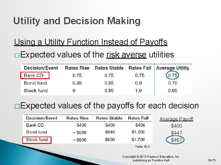
Utility and Decision Making Using a Utility Function Instead of Payoffs � Expected values of the risk averse utilities � Expected values of the payoffs for each decision Average Payoff $400 $447 $467 Table 18. 2 Copyright © 2013 Pearson Education, Inc. publishing as Prentice Hall 18 -73

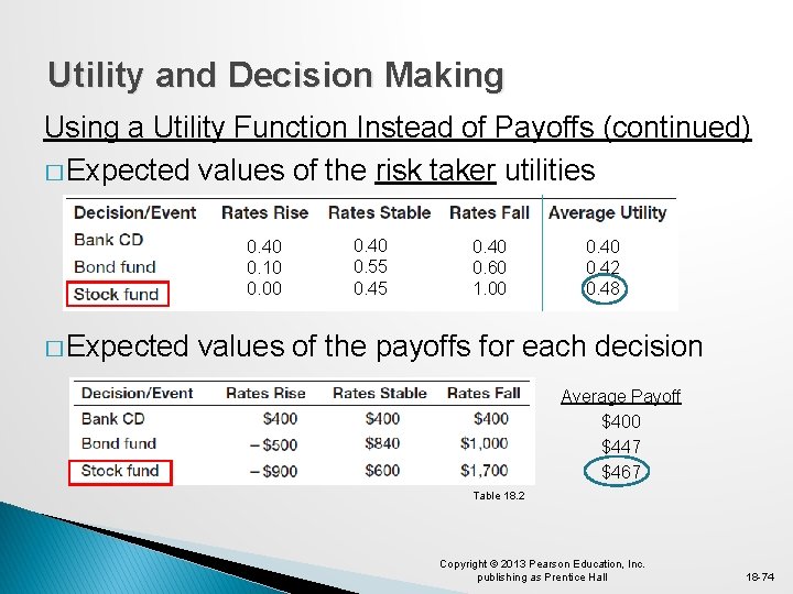
Utility and Decision Making Using a Utility Function Instead of Payoffs (continued) � Expected values of the risk taker utilities 0. 40 0. 10 0. 00 � Expected 0. 40 0. 55 0. 40 0. 60 1. 00 0. 42 0. 48 values of the payoffs for each decision Average Payoff $400 $447 $467 Table 18. 2 Copyright © 2013 Pearson Education, Inc. publishing as Prentice Hall 18 -74

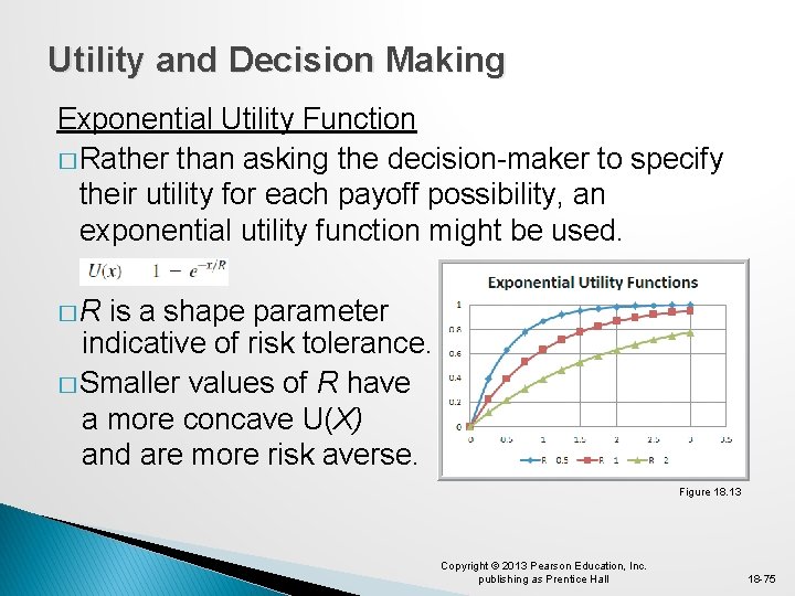
Utility and Decision Making Exponential Utility Function � Rather than asking the decision-maker to specify their utility for each payoff possibility, an exponential utility function might be used. �R is a shape parameter indicative of risk tolerance. � Smaller values of R have a more concave U(X) and are more risk averse. Figure 18. 13 Copyright © 2013 Pearson Education, Inc. publishing as Prentice Hall 18 -75

Utility and Decision Making Exponential Utility Function (continued) One approach to estimating an appropriate value of R for the decision maker is to: � Find the maximum payoff $R for which the decision maker believes that taking a chance to win $R is equivalent to losing $R/2. � Would you take on a bet of possibly winning $10 versus losing $5? � How about risking $50 to win $100? � How about risking $500 to win $1000? � R measures one’s maximum risk comfort level. Copyright © 2013 Pearson Education, Inc. publishing as Prentice Hall 18 -76

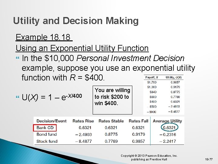
Utility and Decision Making Example 18. 18 Using an Exponential Utility Function In the $10, 000 Personal Investment Decision example, suppose you use an exponential utility function with R = $400. U(X) = 1 – e-X/400 You are willing to risk $200 to win $400. Copyright © 2013 Pearson Education, Inc. publishing as Prentice Hall 18 -77

Utility and Decision Making Analytics in Practice: Using Decision Analysis in Drug Development � Pharma, a business unit of Bayer Pharmaceuticals, developed a new blood-clot-busting drug. � They used a structured decision analysis approach to evaluate market potential of the drug. � A decision tree with 6 decision points delivered to senior managers the expected net present value, the likelihood of success, and the risks involved. � This decision tree approach set new standards for subsequent new drug developments at Pharma. Copyright © 2013 Pearson Education, Inc. publishing as Prentice Hall 18 -78

Chapter 18 - Key Terms Branches Certainty equivalent Decision node Decision strategy Decision tree Event node Expected opportunity loss Expected value of perfect information Expected value of sample information Laplace, or average, payoff strategy Maximax strategy Maximin strategy Copyright © 2013 Pearson Education, Inc. publishing as Prentice Hall 18 -79

Chapter 18 - Key Terms (continued) Minimax regret strategy Minimax strategy Minimin strategy Nodes Payoff table Perfect information Risk averse Risk premium Risk profile Sample information Utility theory Value of information Copyright © 2013 Pearson Education, Inc. publishing as Prentice Hall 18 -80

Case Study Performance Lawn Equipment (18) Recall that PLE produces lawnmowers and a medium size diesel power lawn tractor. PLE has developed a prototype for a new snow blower to help balance its seasonal demand. Management needs to decide whether to introduce the product globally or just in the North American market. You need to construct a decision tree, determine the optimal strategy, and develop a risk profile. Write a formal report summarizing your results. Copyright © 2013 Pearson Education, Inc. publishing as Prentice Hall 18 -81