Using Corpora for Language Research COGS 523 Lecture

Using Corpora for Language Research COGS 523 -Lecture 7 Statistics for Corpora Based Studies 15. 10. 2021 COGS 523 - Bilge Say 1

Related Readings Statistics: • Mc. Enery and Wilson (2001) Ch 3; Mc. Enery et al. (2006) Unit A 6. • For further reading, • • consult Oakes (1998), Chs 1 and 2 Gries, S. (2009). Quantitative Corpus Linguistics with R: a Practical Introduction Jurafsky and Martin (2009) Speech and Language Processing. 2 nd Edition POS tagging example is from Jurafsky’s Lecture Slides (LING 180, Autumn 2006) 15. 10. 2021 COGS 523 - Bilge Say 2

Statistical Analysis n n Descriptive vs. inferential statistics (a subbranch is Bayesian) Objectivist (Frequentist) vs. Subjectivist (Bayesian) Probabilities: n Objectivist: probabilities are real aspects of the world that can be measured by the relative frequencies of outcomes of experiments n Subjectivist: probabilities are descriptions of an observer’s degree of belief or uncertainty rather than having any external significance 15. 10. 2021 COGS 523 - Bilge Say 3

Nature of Corpora In corpus analysis, much of the data is skewed, or very irregular. ex: Number of letters in a word, the length of syllables n Partial solutions: use nonparametric tests (do not assume the normal distribution) disadvantages: less prior information, more training needed in statistical NLP. n Lognormal distributions: analyze a suitably large corpus according to sentence lengths, and produce a graph showing how often each sentence length occurs. n 15. 10. 2021 COGS 523 - Bilge Say 4

Some points to consider n n Quantitative and qualitative Analysis is usually complementary – not a replacement for each other Randomness to sampling is different from measurement errors (automatic annotation etc. ) You have to operationalize your research problem well. Another, different use of statistics: language competence has a probabilistic component 15. 10. 2021 COGS 523 - Bilge Say 5

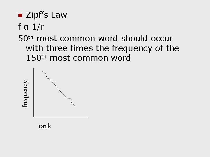
Zipf’s Law f α 1/r 50 th most common word should occur with three times the frequency of the 150 th most common word frequency n rank

Hypothesis testing How likely is it that what you are seeing is statistically significant? ex: In Brown corpus mean sentence length in government documents is 25. 48 words. on corpus as a whole is 19. 27 words. The sentences in government documents are longer than those found in general texts or The observed differences are purely due to chance (null hypothesis) Small effect sizes may lead to highly significant rejection of null hypothesis due to sample sizes in corpora 15. 10. 2021 COGS 523 - Bilge Say 7

The Sample and the Population Make generalizations about a large existing population, such as corpus, without testing it in its entirety n Do the samples exhibit the characteristics of the whole corpus? Test n Compare two existing samples to see whether their statistical behavior is consistent with that expected for two samples drawn from the same hypothetical corpus – more common in linguistics. Ex: authorship studies - corpus of disputed work -controversial text hypothetical corpus: everything the author could have written n n 15. 10. 2021 COGS 523 - Bilge Say 8

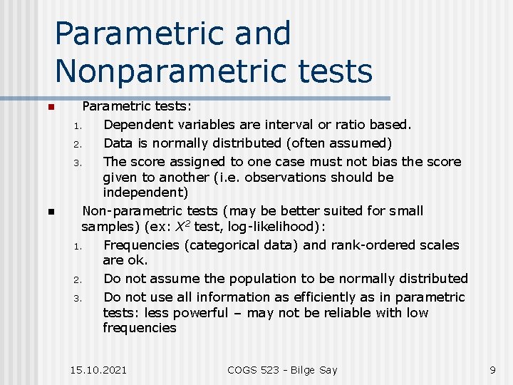
Parametric and Nonparametric tests n n Parametric tests: 1. Dependent variables are interval or ratio based. 2. Data is normally distributed (often assumed) 3. The score assigned to one case must not bias the score given to another (i. e. observations should be independent) Non-parametric tests (may be better suited for small samples) (ex: X 2 test, log-likelihood): 1. Frequencies (categorical data) and rank-ordered scales are ok. 2. Do not assume the population to be normally distributed 3. Do not use all information as efficiently as in parametric tests: less powerful – may not be reliable with low frequencies 15. 10. 2021 COGS 523 - Bilge Say 9

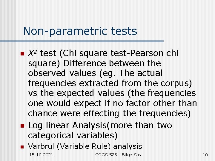
Non-parametric tests n n n X 2 test (Chi square test-Pearson chi square) Difference between the observed values (eg. The actual frequencies extracted from the corpus) vs the expected values (the frequencies one would expect if no factor other than chance were effecting the frequencies) Log linear Analysis(more than two categorical variables) Varbrul (Variable Rule) analysis 15. 10. 2021 COGS 523 - Bilge Say 10

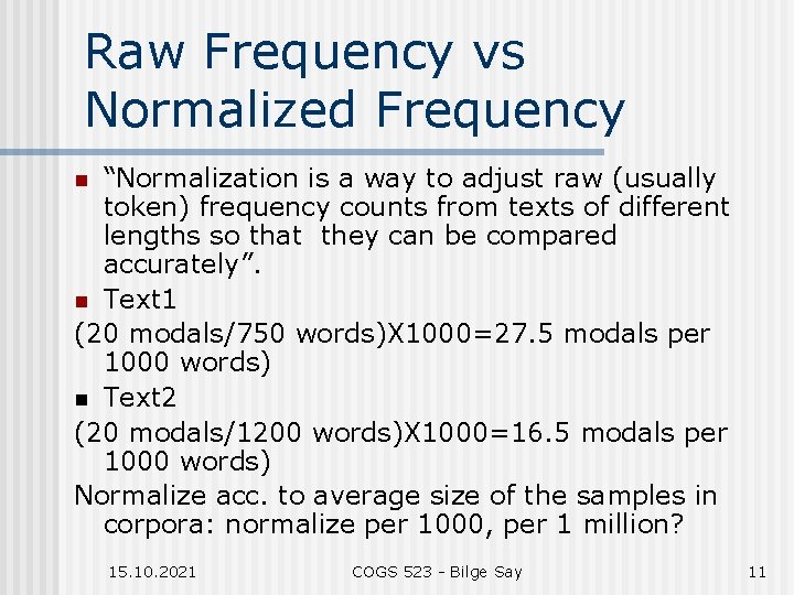
Raw Frequency vs Normalized Frequency “Normalization is a way to adjust raw (usually token) frequency counts from texts of different lengths so that they can be compared accurately”. n Text 1 (20 modals/750 words)X 1000=27. 5 modals per 1000 words) n Text 2 (20 modals/1200 words)X 1000=16. 5 modals per 1000 words) Normalize acc. to average size of the samples in corpora: normalize per 1000, per 1 million? n 15. 10. 2021 COGS 523 - Bilge Say 11

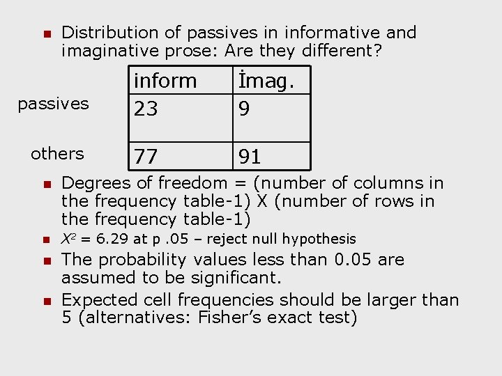
n Distribution of passives in informative and imaginative prose: Are they different? passives others inform 23 İmag. 9 77 91 n Degrees of freedom = (number of columns in the frequency table-1) X (number of rows in the frequency table-1) n X 2 = 6. 29 at p. 05 – reject null hypothesis n The probability values less than 0. 05 are assumed to be significant. Expected cell frequencies should be larger than 5 (alternatives: Fisher’s exact test) n

Factor Analysis n n Variations: Principal Component Analysis, Latent Semantic Analysis, Cluster Analysis A multivariate technique for identifying whether the correlations between a set of observed variables stem from their relationships to one or more latent variables. Group together variables that are distributed in similar ways. Factors (dimensions), Factor loadings, Factor scores 15. 10. 2021 COGS 523 - Bilge Say 13

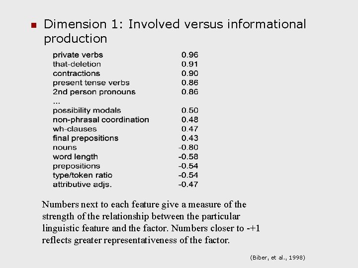
n Dimension 1: Involved versus informational production Numbers next to each feature give a measure of the strength of the relationship between the particular linguistic feature and the factor. Numbers closer to -+1 reflects greater representativeness of the factor. (Biber, et al. , 1998)

Basics of Bayesian Statistics Notions of joint probability, conditional probability n Bayes’ Rule n Information Theory n Applications in Computational and Theoretical Linguistics. . . n Not intended as a full treatment. . . n 15. 10. 2021 COGS 523 - Bilge Say 15

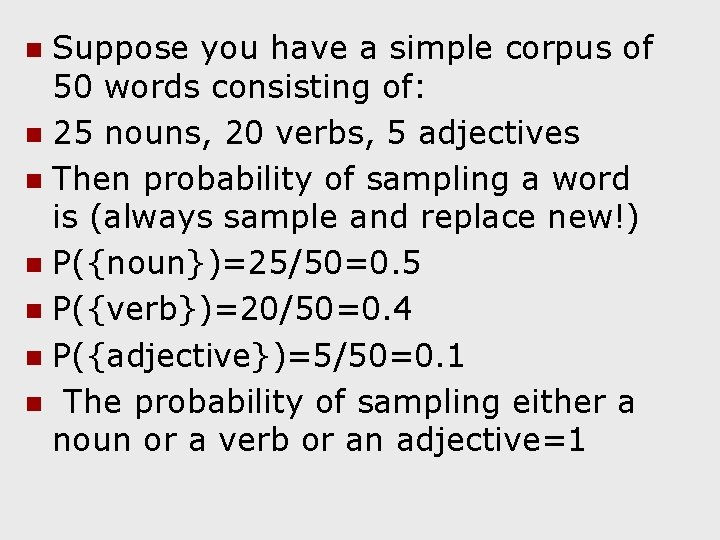
Suppose you have a simple corpus of 50 words consisting of: n 25 nouns, 20 verbs, 5 adjectives n Then probability of sampling a word is (always sample and replace new!) n P({noun})=25/50=0. 5 n P({verb})=20/50=0. 4 n P({adjective})=5/50=0. 1 n The probability of sampling either a noun or a verb or an adjective=1 n

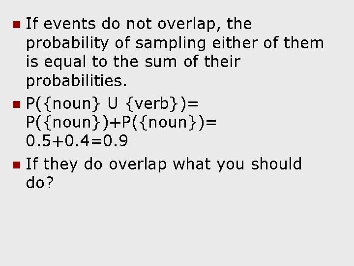
If events do not overlap, the probability of sampling either of them is equal to the sum of their probabilities. n P({noun} U {verb})= P({noun})+P({noun})= 0. 5+0. 4=0. 9 n If they do overlap what you should do? n

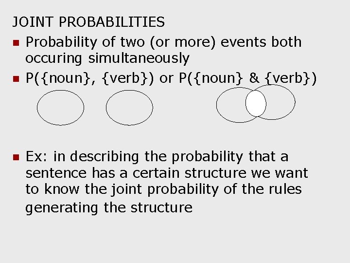
JOINT PROBABILITIES n Probability of two (or more) events both occuring simultaneously n P({noun}, {verb}) or P({noun} & {verb}) n Ex: in describing the probability that a sentence has a certain structure we want to know the joint probability of the rules generating the structure

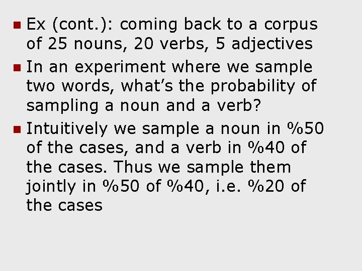
Ex (cont. ): coming back to a corpus of 25 nouns, 20 verbs, 5 adjectives n In an experiment where we sample two words, what’s the probability of sampling a noun and a verb? n Intuitively we sample a noun in %50 of the cases, and a verb in %40 of the cases. Thus we sample them jointly in %50 of %40, i. e. %20 of the cases n

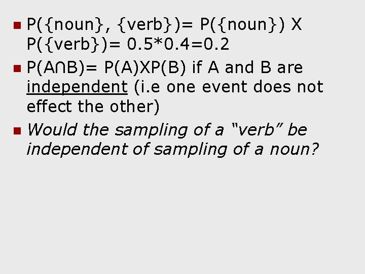
P({noun}, {verb})= P({noun}) X P({verb})= 0. 5*0. 4=0. 2 n P(A∩B)= P(A)XP(B) if A and B are independent (i. e one event does not effect the other) n Would the sampling of a “verb” be independent of sampling of a noun? n

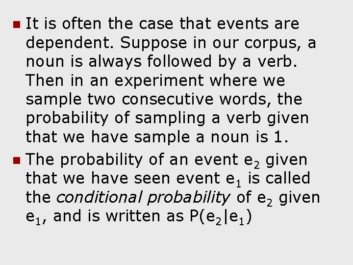
It is often the case that events are dependent. Suppose in our corpus, a noun is always followed by a verb. Then in an experiment where we sample two consecutive words, the probability of sampling a verb given that we have sample a noun is 1. n The probability of an event e 2 given that we have seen event e 1 is called the conditional probability of e 2 given e 1, and is written as P(e 2|e 1) n

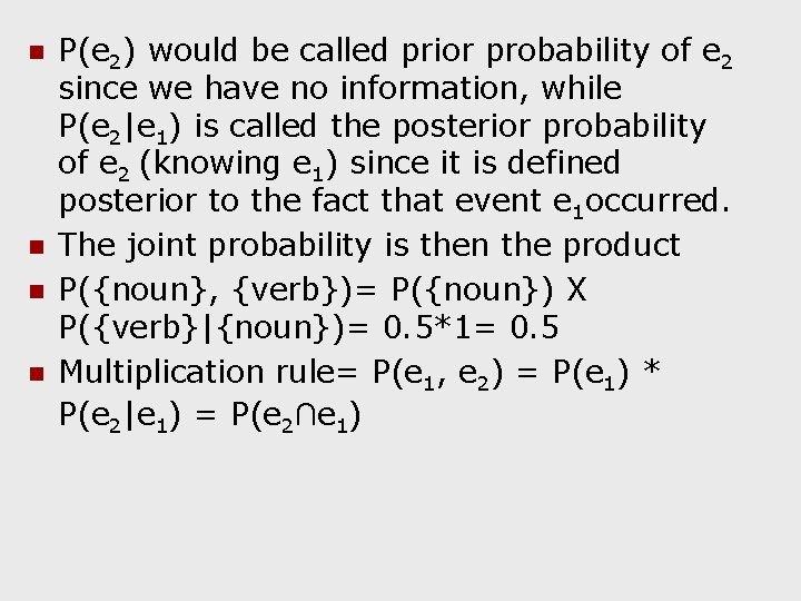
n n P(e 2) would be called prior probability of e 2 since we have no information, while P(e 2|e 1) is called the posterior probability of e 2 (knowing e 1) since it is defined posterior to the fact that event e 1 occurred. The joint probability is then the product P({noun}, {verb})= P({noun}) X P({verb}|{noun})= 0. 5*1= 0. 5 Multiplication rule= P(e 1, e 2) = P(e 1) * P(e 2|e 1) = P(e 2∩e 1)

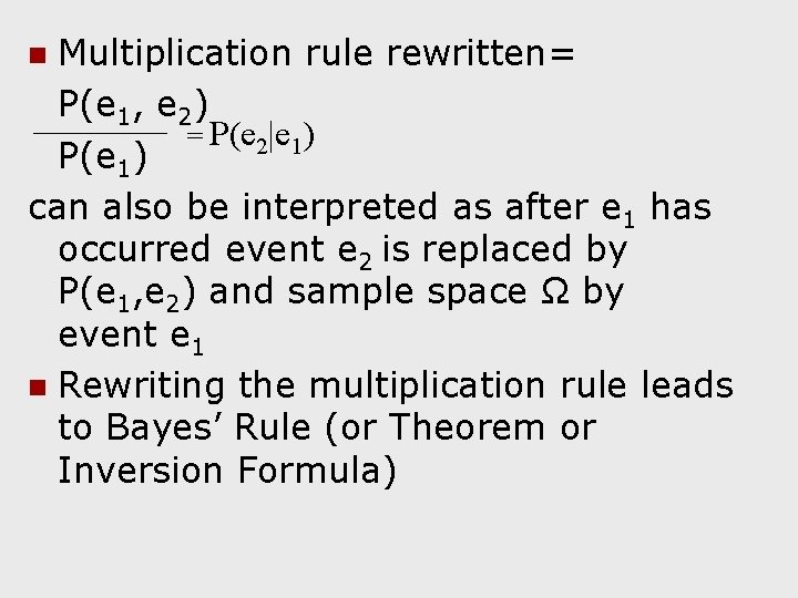
Multiplication rule rewritten= P(e 1, e 2) = P(e 2|e 1) P(e 1) can also be interpreted as after e 1 has occurred event e 2 is replaced by P(e 1, e 2) and sample space Ω by event e 1 n Rewriting the multiplication rule leads to Bayes’ Rule (or Theorem or Inversion Formula) n

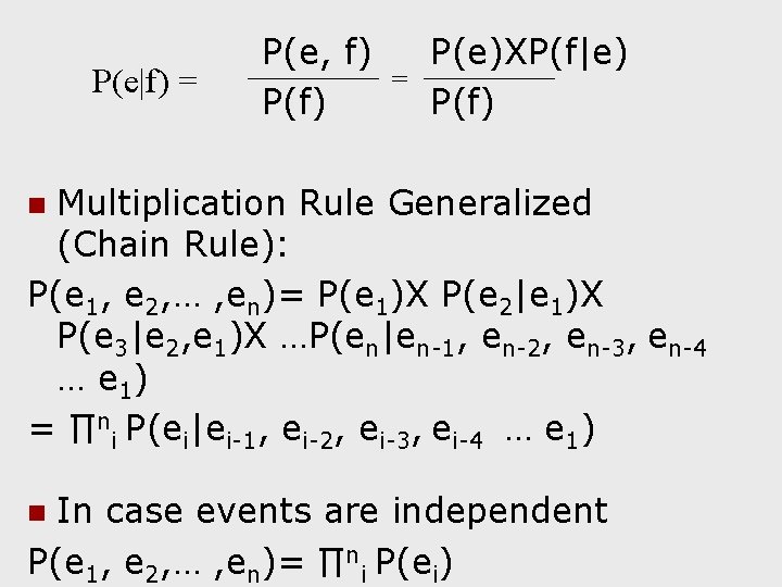
P(e|f) = P(e, f) P(f) = P(e)XP(f|e) P(f) Multiplication Rule Generalized (Chain Rule): P(e 1, e 2, … , en)= P(e 1)X P(e 2|e 1)X P(e 3|e 2, e 1)X …P(en|en-1, en-2, en-3, en-4 … e 1) = ∏ni P(ei|ei-1, ei-2, ei-3, ei-4 … e 1) n In case events are independent P(e 1, e 2, … , en)= ∏ni P(ei) n

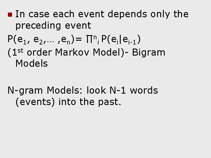
In case each event depends only the preceding event P(e 1, e 2, … , en)= ∏ni P(ei|ei-1) (1 st order Markov Model)- Bigram Models n N-gram Models: look N-1 words (events) into the past.

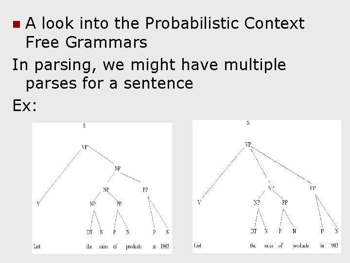
A look into the Probabilistic Context Free Grammars In parsing, we might have multiple parses for a sentence Ex: n

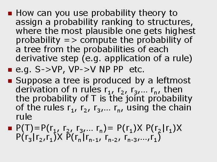
n n How can you use probability theory to assign a probability ranking to structures, where the most plausible one gets highest probability => compute the probability of a tree from the probabilities of each derivative step (e. g. application of a rule) e. g. S->VP, VP->V NP PP etc. Suppose a tree is produced by a leftmost derivation of n rules r 1, r 2, r 3, … rn, then the probability of T is the joint probability of the rules r 1, r 2, r 3, … rn, using the chain rule P(T)=P(r 1, r 2, r 3, … rn)= P(r 1)X P(r 2|r 1)X P(r 3|r 2, r 1)X P(rn|rn-1, rn-2, rn-3, …, r 1)

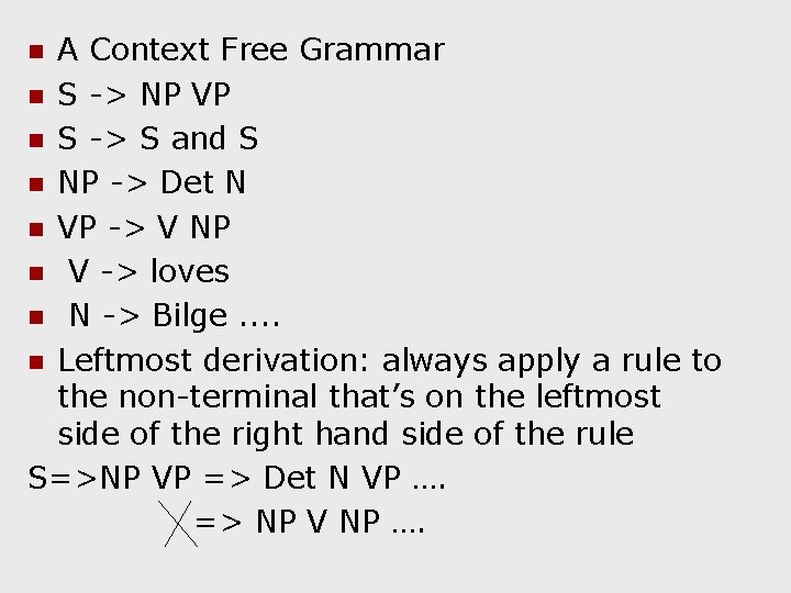
A Context Free Grammar n S -> NP VP n S -> S and S n NP -> Det N n VP -> V NP n V -> loves n N -> Bilge. . n Leftmost derivation: always apply a rule to the non-terminal that’s on the leftmost side of the right hand side of the rule S=>NP VP => Det N VP …. => NP V NP …. n

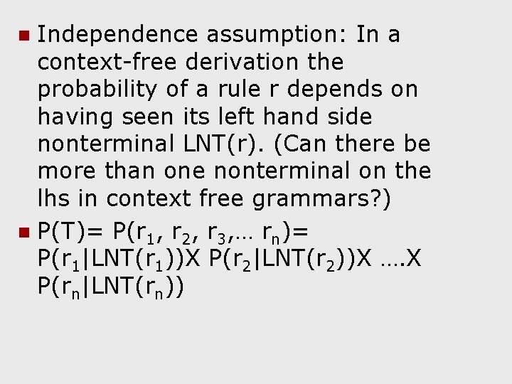
Independence assumption: In a context-free derivation the probability of a rule r depends on having seen its left hand side nonterminal LNT(r). (Can there be more than one nonterminal on the lhs in context free grammars? ) n P(T)= P(r 1, r 2, r 3, … rn)= P(r 1|LNT(r 1))X P(r 2|LNT(r 2))X …. X P(rn|LNT(rn)) n

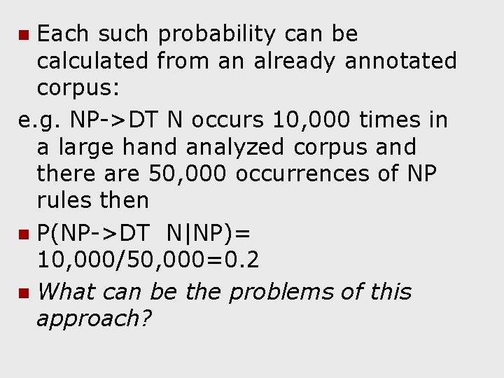
Each such probability can be calculated from an already annotated corpus: e. g. NP->DT N occurs 10, 000 times in a large hand analyzed corpus and there are 50, 000 occurrences of NP rules then n P(NP->DT N|NP)= 10, 000/50, 000=0. 2 n What can be the problems of this approach? n

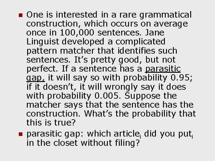
n n One is interested in a rare grammatical construction, which occurs on average once in 100, 000 sentences. Jane Linguist developed a complicated pattern matcher that identifies such sentences. It’s pretty good, but not perfect. If a sentence has a parasitic gap, it will say so with probability 0. 95; if it doesn’t, it will wrongly say it does with probability 0. 005. Suppose the matcher says that the sentence has the construction. What’s the probability that this is true? parasitic gap: which articlei did you puti in the closet without filing?

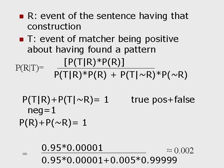
R: event of the sentence having that construction n T: event of matcher being positive about having found a pattern [P(T|R)*P(R)] P(R|T)= P(T|R)*P(R) + P(T|~R)*P(~R) n P(T|R)+P(T|~R)= 1 neg=1 P(R)+P(~R)= 1 = true pos+false 0. 95*0. 00001 ≈ 0. 002 0. 95*0. 00001+0. 005*0. 99999

n n On average only 1 in every 500 sentences the test identifies, will actually contain the rare construction. This is actually very low due to low prior probability of R – a common cognitive fallacy: base rate neglect. . .

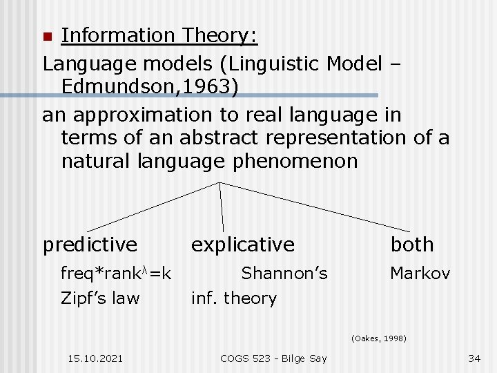
Information Theory: Language models (Linguistic Model – Edmundson, 1963) an approximation to real language in terms of an abstract representation of a natural language phenomenon n predictive freq*rankλ=k Zipf’s law explicative both Shannon’s inf. theory Markov (Oakes, 1998) 15. 10. 2021 COGS 523 - Bilge Say 34

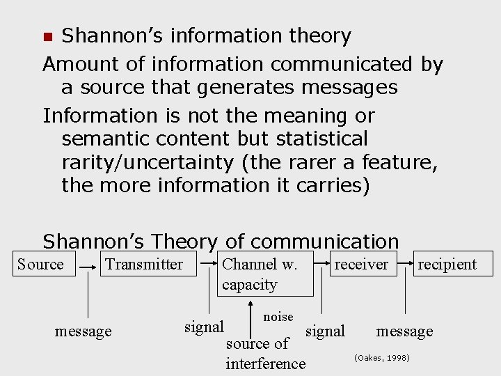
Shannon’s information theory Amount of information communicated by a source that generates messages Information is not the meaning or semantic content but statistical rarity/uncertainty (the rarer a feature, the more information it carries) n Shannon’s Theory of communication Source Transmitter message Channel w. capacity signal noise receiver signal source of interference recipient message (Oakes, 1998)

Stochastic Process: a physical system or a mathematical model of a system, which produces a sequence of symbols governed by a set of probabilities n Language as a code: an alphabet of elementary symbols with rules for combination continuous messages vs. discrete messages (speech) (written text) n

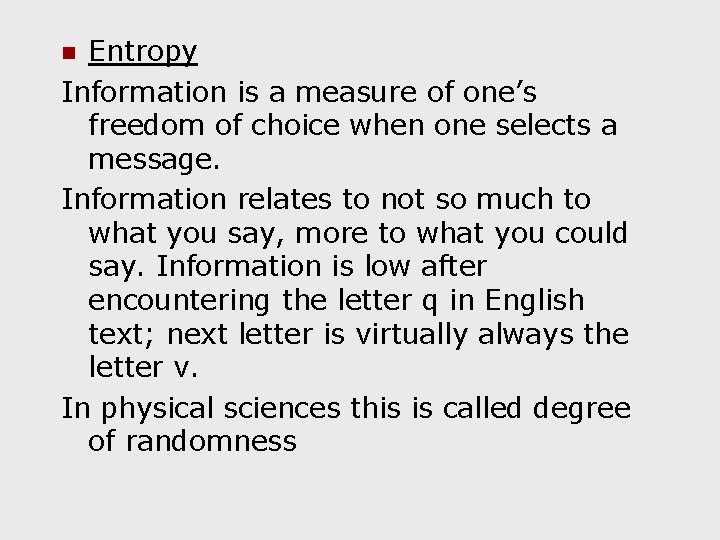
Entropy Information is a measure of one’s freedom of choice when one selects a message. Information relates to not so much to what you say, more to what you could say. Information is low after encountering the letter q in English text; next letter is virtually always the letter v. In physical sciences this is called degree of randomness n

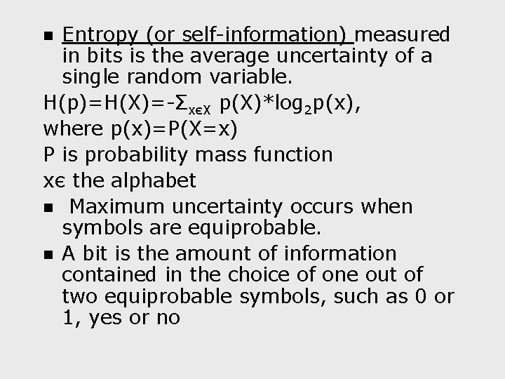
Entropy (or self-information) measured in bits is the average uncertainty of a single random variable. H(p)=H(X)=-ΣxєX p(X)*log 2 p(x), where p(x)=P(X=x) P is probability mass function xє the alphabet n Maximum uncertainty occurs when symbols are equiprobable. n A bit is the amount of information contained in the choice of one out of two equiprobable symbols, such as 0 or 1, yes or no n

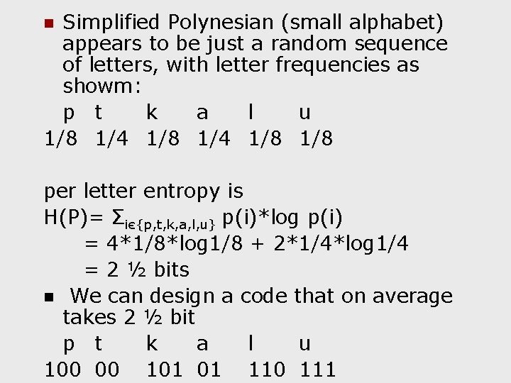
Simplified Polynesian (small alphabet) appears to be just a random sequence of letters, with letter frequencies as showm: p t k a l u 1/8 1/4 1/8 n per letter entropy is H(P)= Σiє{p, t, k, a, l, u} p(i)*log p(i) = 4*1/8*log 1/8 + 2*1/4*log 1/4 = 2 ½ bits n We can design a code that on average takes 2 ½ bit p t k a l u 100 00 101 01 110 111

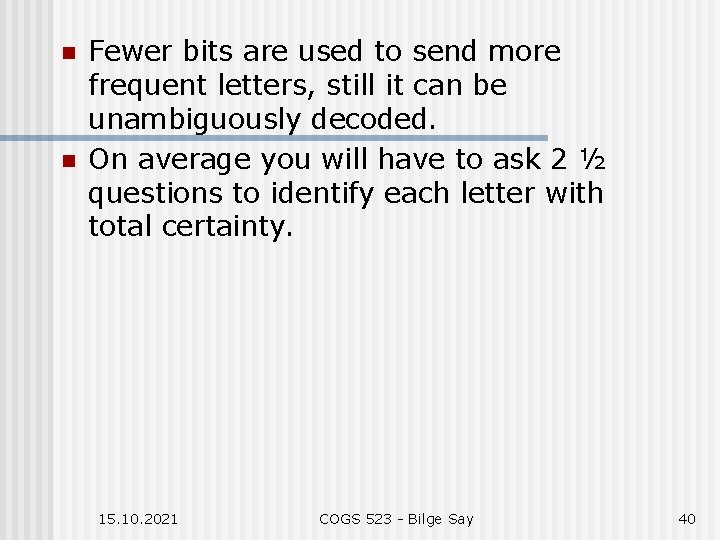
n n Fewer bits are used to send more frequent letters, still it can be unambiguously decoded. On average you will have to ask 2 ½ questions to identify each letter with total certainty. 15. 10. 2021 COGS 523 - Bilge Say 40

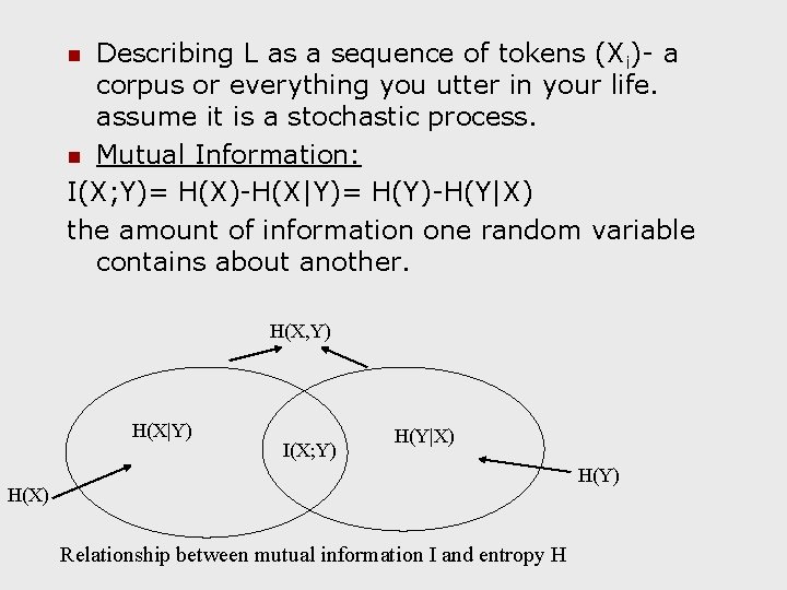
Describing L as a sequence of tokens (Xi)- a corpus or everything you utter in your life. assume it is a stochastic process. n Mutual Information: I(X; Y)= H(X)-H(X|Y)= H(Y)-H(Y|X) the amount of information one random variable contains about another. n H(X, Y) H(X|Y) I(X; Y) H(Y|X) H(Y) H(X) Relationship between mutual information I and entropy H

n n How would entropy (using English alphabet) change (increase/decrease) as you go from letters to trigrams? The conditional entropy: of a discrete random variable Y given another X, for X, Y ~p(X, Y) expresses how much extra info. you still need to supply on average to communicate Y given that receiver knows X.

Mutual Information (cont. ): Reduction in uncertainty of one random variable due to knowing about another (used in studying collocations- how likely are they to appear together within a span of words, e. g. a window of three words? ) n n Practical Applications (in NLP) clustering word sense disambiguation; word segmentation in Chinese, collocations – MI > 3 – good indication of collocational strength (z and t scores are also used)

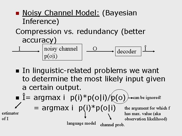
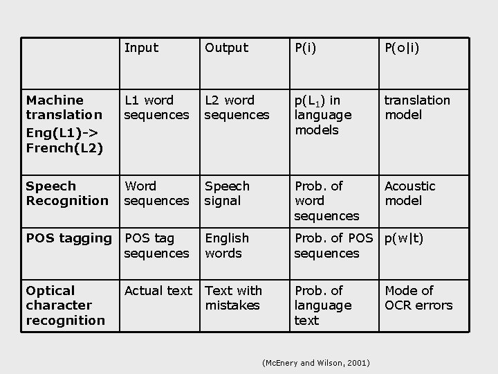
Noisy Channel Model: (Bayesian Inference) Compression vs. redundancy (better accuracy) n I n n estimator of I noisy channel p(o|i) O decoder Î In linguistic-related problems we want to determine the most likely input given a certain output. Î= argmax i p(i)*p(o|i)/p(o) can be ignored! = argmax i p(i)*p(o|i) the argument for which f has max. value (aka observation likelihood) language model channel prob.

Input Output P(i) P(o|i) Machine translation Eng(L 1)-> French(L 2) L 1 word sequences L 2 word sequences p(L 1) in language models translation model Speech Recognition Word sequences Speech signal Prob. of word sequences Acoustic model POS tagging POS tag sequences English words Prob. of POS p(w|t) sequences Optical character recognition Actual text Text with mistakes Prob. of language text (Mc. Enery and Wilson, 2001) Mode of OCR errors

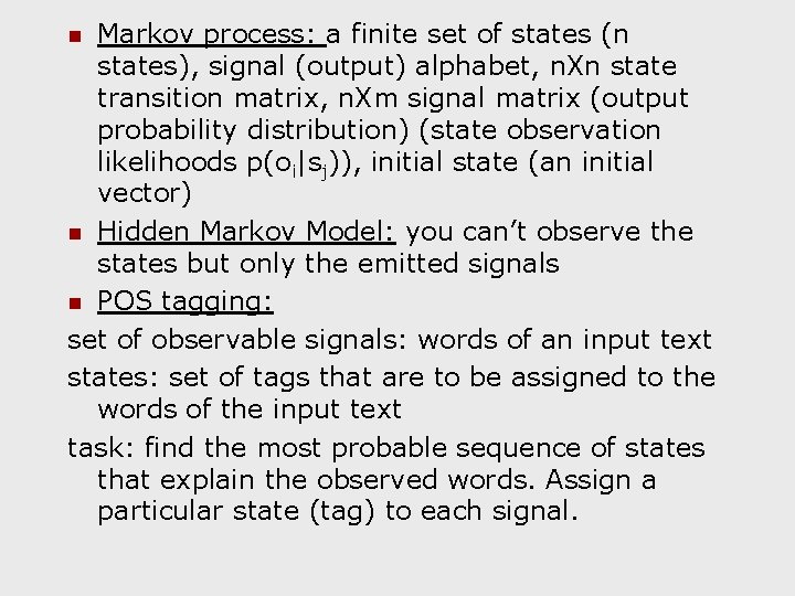
Markov process: a finite set of states (n states), signal (output) alphabet, n. Xn state transition matrix, n. Xm signal matrix (output probability distribution) (state observation likelihoods p(oi|sj)), initial state (an initial vector) n Hidden Markov Model: you can’t observe the states but only the emitted signals n POS tagging: set of observable signals: words of an input text states: set of tags that are to be assigned to the words of the input text task: find the most probable sequence of states that explain the observed words. Assign a particular state (tag) to each signal. n

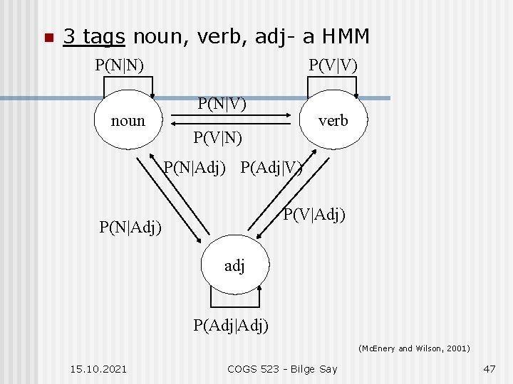
n 3 tags noun, verb, adj- a HMM P(N|N) noun P(V|V) P(N|V) verb P(V|N) P(N|Adj) P(Adj|V) P(V|Adj) P(N|Adj) adj P(Adj|Adj) (Mc. Enery and Wilson, 2001) 15. 10. 2021 COGS 523 - Bilge Say 47

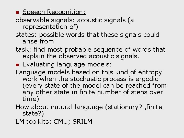
Speech Recognition: observable signals: acoustic signals (a representation of) states: possible words that these signals could arise from task: find most probable sequence of words that explain the observed acoustic signals. n Evaluating language models: Language models based on this kind of entropy work when the stochastic process is ergodic (every state of the model can be reached from any other state in finite number of steps over time) How about natural language (stationary? , finite state? ) LM toolkits: CMU; SRILM n

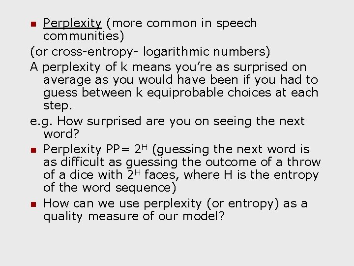
Perplexity (more common in speech communities) (or cross-entropy- logarithmic numbers) A perplexity of k means you’re as surprised on average as you would have been if you had to guess between k equiprobable choices at each step. e. g. How surprised are you on seeing the next word? n Perplexity PP= 2 H (guessing the next word is as difficult as guessing the outcome of a throw of a dice with 2 H faces, where H is the entropy of the word sequence) n How can we use perplexity (or entropy) as a quality measure of our model? n

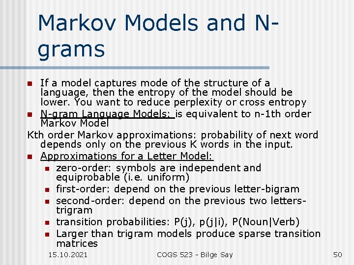
Markov Models and Ngrams If a model captures mode of the structure of a language, then the entropy of the model should be lower. You want to reduce perplexity or cross entropy n N-gram Language Models: is equivalent to n-1 th order Markov Model Kth order Markov approximations: probability of next word depends only on the previous K words in the input. n Approximations for a Letter Model: n zero-order: symbols are independent and equiprobable (i. e. uniform) n first-order: depend on the previous letter-bigram n second-order: depend on the previous two letterstrigram n transition probabilities: P(j), p(j|i), P(Noun|Verb) n Larger than trigram models produce sparse transition matrices n 15. 10. 2021 COGS 523 - Bilge Say 50

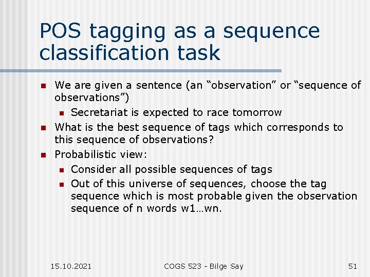
POS tagging as a sequence classification task n n n We are given a sentence (an “observation” or “sequence of observations”) n Secretariat is expected to race tomorrow What is the best sequence of tags which corresponds to this sequence of observations? Probabilistic view: n Consider all possible sequences of tags n Out of this universe of sequences, choose the tag sequence which is most probable given the observation sequence of n words w 1…wn. 15. 10. 2021 COGS 523 - Bilge Say 51

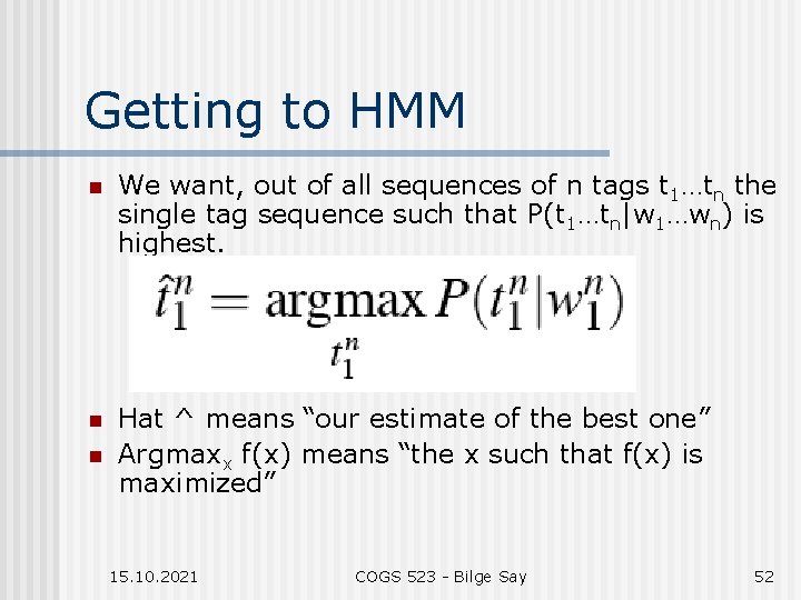
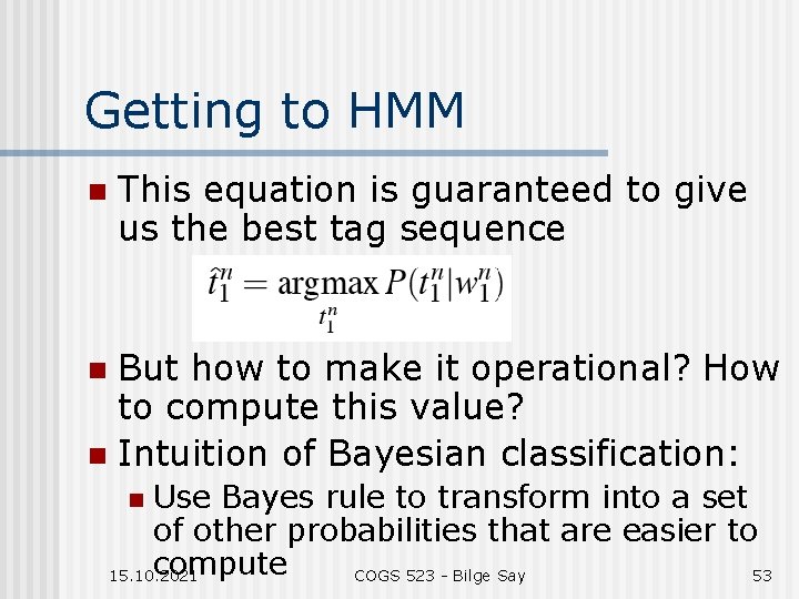
Getting to HMM n We want, out of all sequences of n tags t 1…tn the single tag sequence such that P(t 1…tn|w 1…wn) is highest. n Hat ^ means “our estimate of the best one” Argmaxx f(x) means “the x such that f(x) is maximized” n 15. 10. 2021 COGS 523 - Bilge Say 52

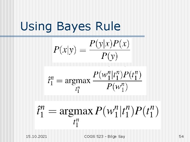
Getting to HMM n This equation is guaranteed to give us the best tag sequence But how to make it operational? How to compute this value? n Intuition of Bayesian classification: n Use Bayes rule to transform into a set of other probabilities that are easier to compute 15. 10. 2021 COGS 523 - Bilge Say 53 n

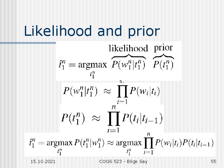
Using Bayes Rule 15. 10. 2021 COGS 523 - Bilge Say 54

Likelihood and prior n 15. 10. 2021 COGS 523 - Bilge Say 55

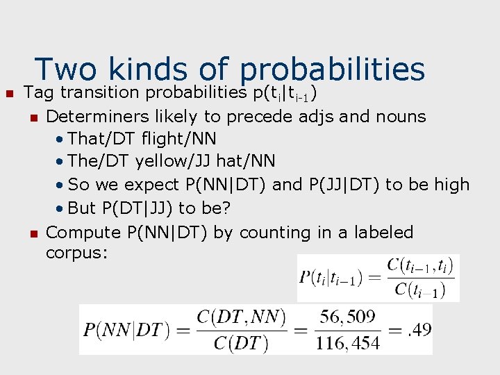
Two kinds of probabilities n Tag transition probabilities p(ti|ti-1) n Determiners likely to precede adjs and nouns • That/DT flight/NN • The/DT yellow/JJ hat/NN • So we expect P(NN|DT) and P(JJ|DT) to be high • But P(DT|JJ) to be? n Compute P(NN|DT) by counting in a labeled corpus:

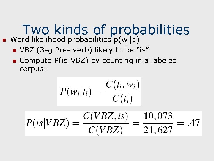
Two kinds of probabilities n Word likelihood probabilities p(wi|ti) n VBZ (3 sg Pres verb) likely to be “is” n Compute P(is|VBZ) by counting in a labeled corpus:

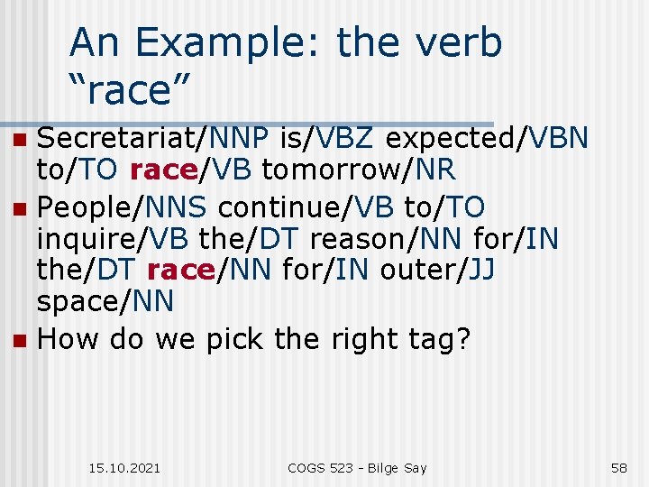
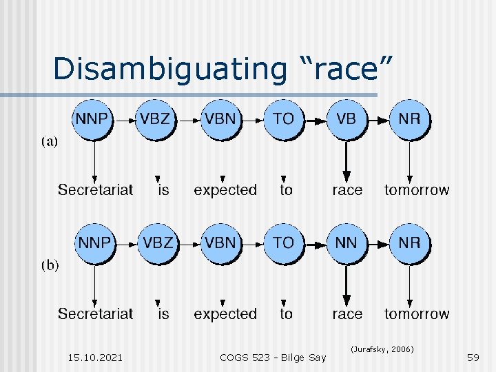
An Example: the verb “race” Secretariat/NNP is/VBZ expected/VBN to/TO race/VB tomorrow/NR n People/NNS continue/VB to/TO inquire/VB the/DT reason/NN for/IN the/DT race/NN for/IN outer/JJ space/NN n How do we pick the right tag? n 15. 10. 2021 COGS 523 - Bilge Say 58

Disambiguating “race” 15. 10. 2021 COGS 523 - Bilge Say (Jurafsky, 2006) 59

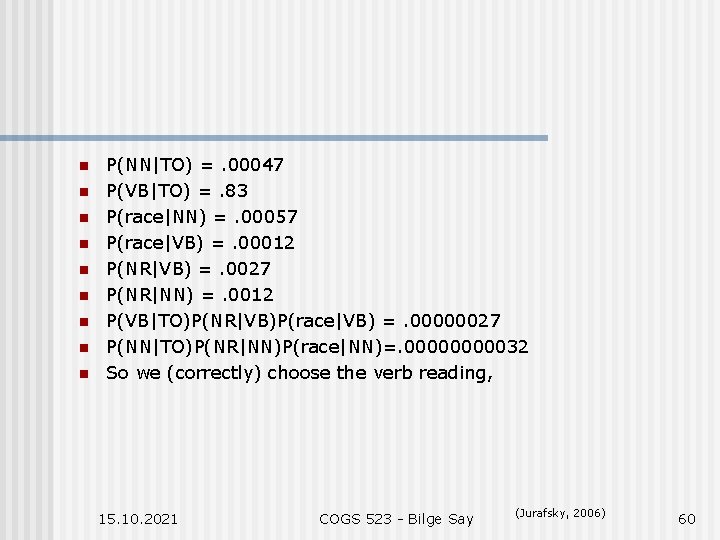
n n n n n P(NN|TO) =. 00047 P(VB|TO) =. 83 P(race|NN) =. 00057 P(race|VB) =. 00012 P(NR|VB) =. 0027 P(NR|NN) =. 0012 P(VB|TO)P(NR|VB)P(race|VB) =. 00000027 P(NN|TO)P(NR|NN)P(race|NN)=. 0000032 So we (correctly) choose the verb reading, 15. 10. 2021 COGS 523 - Bilge Say (Jurafsky, 2006) 60

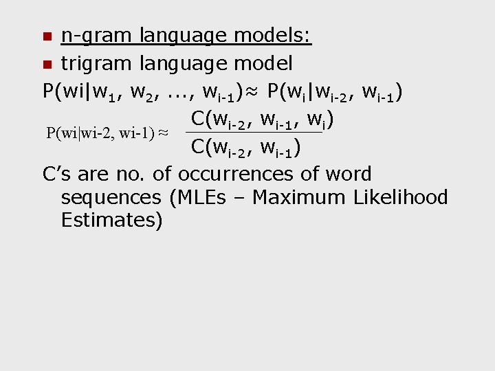
n-gram language models: n trigram language model P(wi|w 1, w 2, . . . , wi-1)≈ P(wi|wi-2, wi-1) C(wi-2, wi-1, wi) P(wi|wi-2, wi-1) ≈ C(wi-2, wi-1) C’s are no. of occurrences of word sequences (MLEs – Maximum Likelihood Estimates) n

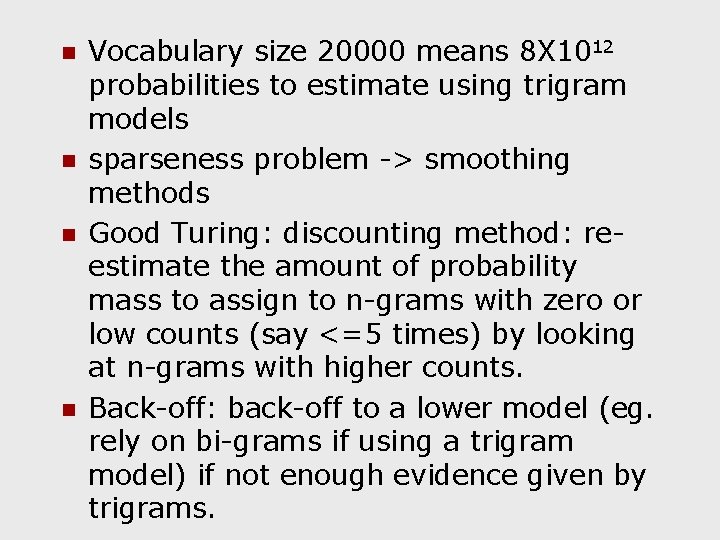
n n Vocabulary size 20000 means 8 X 1012 probabilities to estimate using trigram models sparseness problem -> smoothing methods Good Turing: discounting method: reestimate the amount of probability mass to assign to n-grams with zero or low counts (say <=5 times) by looking at n-grams with higher counts. Back-off: back-off to a lower model (eg. rely on bi-grams if using a trigram model) if not enough evidence given by trigrams.

Next Week Due: Your progress reports n Collocations – Manning and Schutze (1999), Ch 5 n 15. 10. 2021 COGS 523 - Bilge Say 63