Statistical Programming Using the R Language Lecture 1

Statistical Programming Using the R Language Lecture 1 Basic Concepts I Darren J. Fitzpatrick, Ph. D June 2017

Preliminaries • Course will run for 2 hours per day for 5 days (10: 00 – 12: 00). • Broadly divided into: • 1 hour lecture • 1 hour practical/problem sheet • Course website: • http: //bioinf. gen. tcd. ie/workshops/R • Prior to each lecture notes, problem sheets and data will be available at the above address. Solutions will be posted after each lecture. • I can be contacted at the following: • E-mail: fitzptrd@tcd. ie Trinity College Dublin, The University of Dublin

Course Overview I • Lecture 1 – Basic Concepts I • MAC, RStudio, syntax, functions, files and data structures • Lecture 2 – Basic Concepts II • More syntax, plotting, exploratory data analysis • Lecture 3 – Hypothesis Testing • Concepts, normality, F-test, t-test, wilcoxon test, correlation • Lecture 4 – Experimental Design & ANOVA • Power calculations, ANOVA • Lecture 5 – Introducing Multivariate Analysis • Clustering, hierarchical, k-means, heatmaps

Course Overview II • The course is NOT intended to provide comprehensive coverage of either R or statistics. • It is intended to provide: • Adequate fluency in the R language such that users can easily learn additions relevant to their needs. • Familiarity in applying statistics to datasets and interpreting the results. • Take the mystery out of using code. • Mistakes are encouraged – unlike cells, R will neither starve nor die!

Lecture 1 - Overview 1. R – what, where, why? 2. Getting to grips with: – MAC – Rstudio 3. Beginning R programming: • Variables • Data Types • Operators • Functions • Getting help • Dealing with files • Data Structures Trinity College Dublin, The University of Dublin

R – what, why, where? • R is fundamentally a programming language suitable for data analysis • R has ~4000 packages enabling advanced data analytics, exploration and visualisation • Bioconductor a suite of specialised tools for biological data analysis integrates with R • R has a learning curve but once the basics are mastered, it offers flexibility to deal with any imaginable analytics problem.

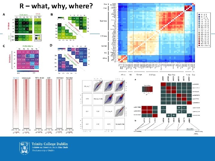
R – what, why, where?

Using a MAC (briefly!) • The main differences between a MAC and a PC • cmd instead of control (e. g. cmd-C for copying) • right click mouse: ctrl-click • # character: alt-3 • switch between applications: cmd-tab • Spotlight (magnifying glass top right): finds files/programs • Apple symbol (top left): for logging out, preferences, etc.

Resources The R Website: https: //www. r-project. org Statistics in R Using Biological Examples: https: //cran. r-project. org/doc/contrib/Seefeld_Stats. RBio. pdf Statistics: an introduction using R http: //www. amazon. co. uk/Statistics-An-Introduction-Using-R/dp/1118941098/ Bioconductor: https: //www. bioconductor. org

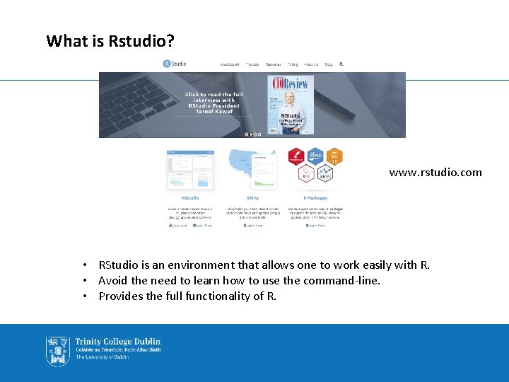
What is Rstudio? www. rstudio. com • RStudio is an environment that allows one to work easily with R. • Avoid the need to learn how to use the command-line. • Provides the full functionality of R.

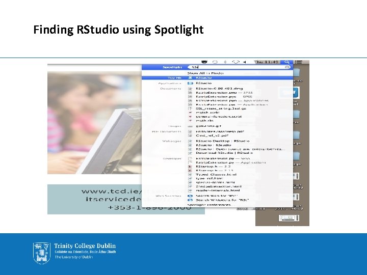
Finding RStudio using Spotlight

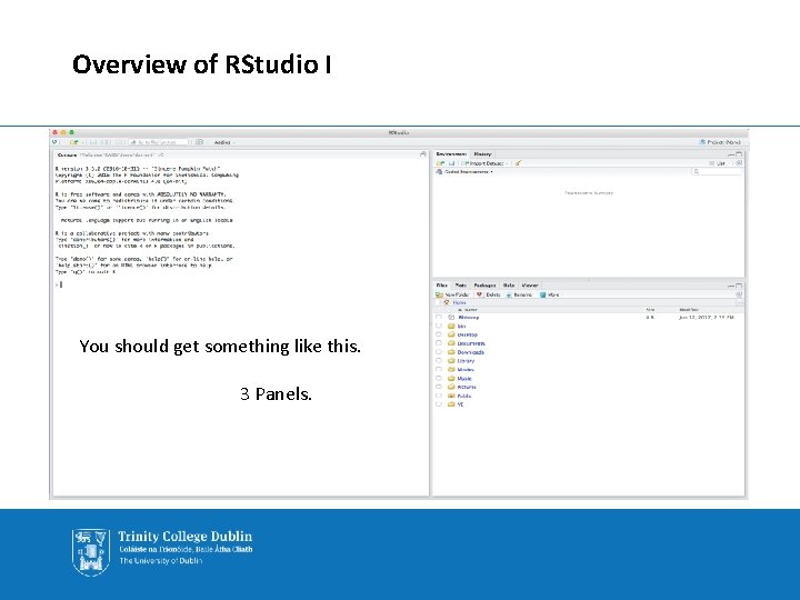
Overview of RStudio I You should get something like this. 3 Panels.

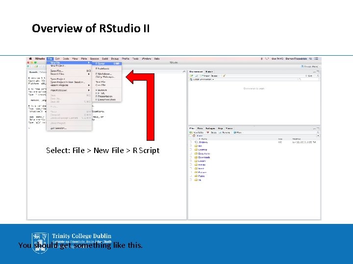
Overview of RStudio II Select: File > New File > R Script You should get something like this.

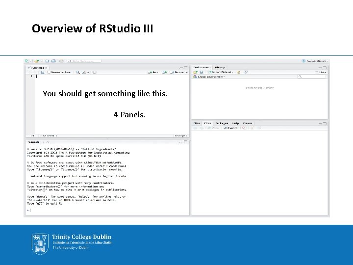
Overview of RStudio III You should get something like this. 4 Panels.

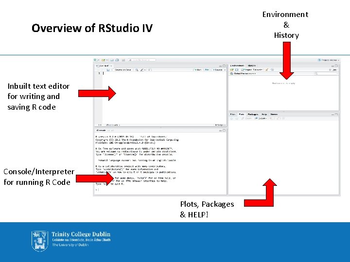
Environment & History Overview of RStudio IV Inbuilt text editor for writing and saving R code Console/Interpreter for running R Code Plots, Packages & HELP!

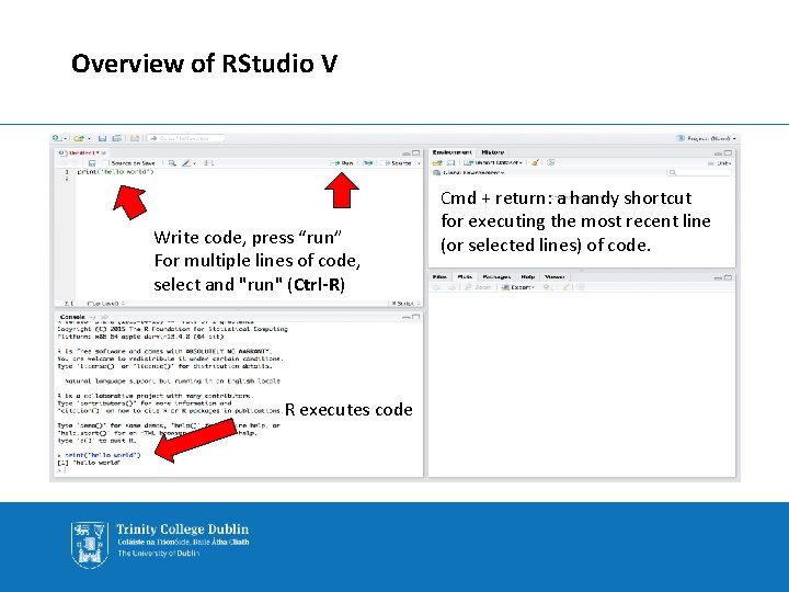
Overview of RStudio V Write code, press “run” For multiple lines of code, select and "run" (Ctrl-R) R executes code Cmd + return: a handy shortcut for executing the most recent line (or selected lines) of code.

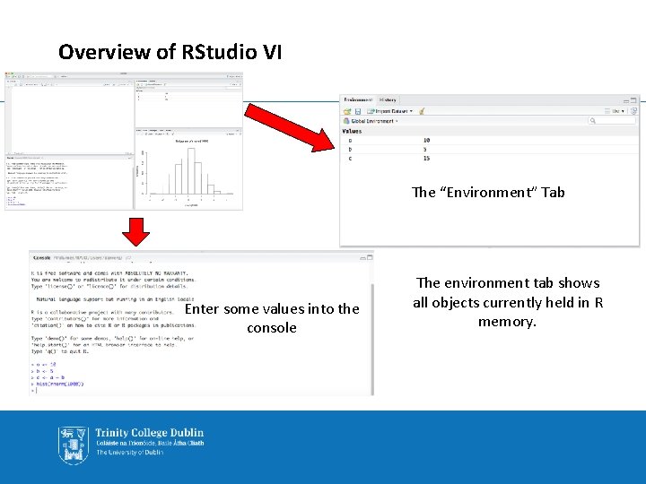
Overview of RStudio VI The “Environment” Tab Enter some values into the console The environment tab shows all objects currently held in R memory.

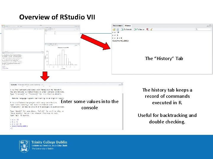
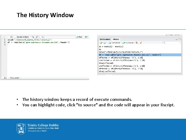
Overview of RStudio VII The “History” Tab “History” Enter some values into the console The history tab keeps a record of commands executed in R. Useful for backtracking and double checking.

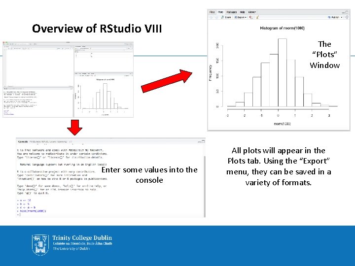
Overview of RStudio VIII The “Plots” Window Enter some values into the console All plots will appear in the Plots tab. Using the “Export” menu, they can be saved in a variety of formats.

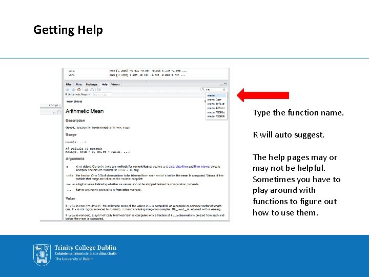
Getting Help Type the function name. R will auto suggest. The help pages may or may not be helpful. Sometimes you have to play around with functions to figure out how to use them.

Basic Syntax of R > print('hello world') > [1] "hello world" • print() is an inbuilt R function • Functions are always of the form function() • Arguments are passed to a function using the brackets • 'hello world' is an argument Trinity College Dublin, The University of Dublin

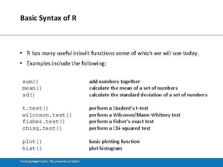
Basic Syntax of R • R has many useful inbuilt functions some of which we will use today. • Examples include the following: sum() mean() sd() add numbers together calculate the mean of a set of numbers calculate the standard deviation of a set of numbers t. test() wilcoxon. test() fisher. test() chisq. test() perform a Student’s t-test perform a Wilcoxon/Mann-Whitney test perform a Fisher’s exact test perform a Chi-squared test plot() hist() basic plotting function plot histogram Trinity College Dublin, The University of Dublin

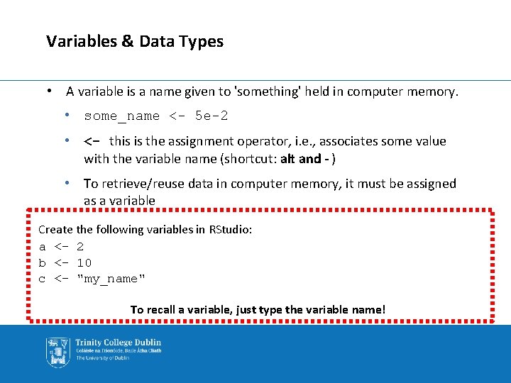
Variables & Data Types • A variable is a name given to 'something' held in computer memory. • some_name <- 5 e-2 • <- this is the assignment operator, i. e. , associates some value with the variable name (shortcut: alt and - ) • To retrieve/reuse data in computer memory, it must be assigned as a variable Create the following variables in RStudio: a <- 2 b <- 10 c <- "my_name" To recall a variable, just type the variable name!

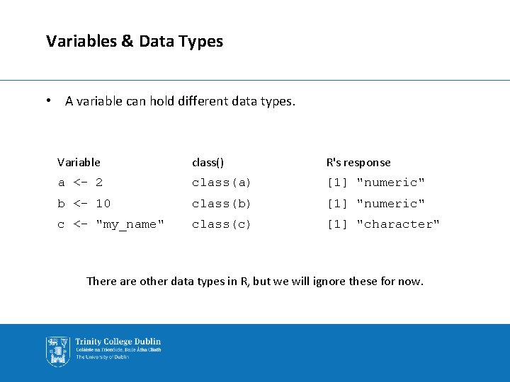
Variables & Data Types • A variable can hold different data types. Variable class() R's response a <- 2 class(a) [1] "numeric" b <- 10 class(b) [1] "numeric" c <- "my_name" class(c) [1] "character" There are other data types in R, but we will ignore these for now.

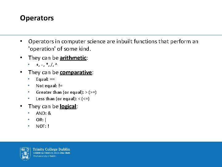
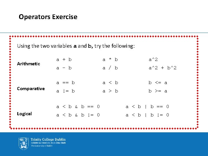
Operators • Operators in computer science are inbuilt functions that perform an 'operation' of some kind. • They can be arithmetic: • +, - , *, /, ^ • They can be comparative: • • Equal: == Not equal: != Greater than (or equal): > (>=) Less than (or equal): < (<=) • They can be logical: • • • AND: & OR: | NOT: !

Operators Exercise Using the two variables a and b, try the following: Arithmetic Comparative Logical a + b a * b a^2 a - b a / b a^2 + b^2 a == b a < b b <= a a != b a > b b >= a a < b & b == 0 a < b | b == 0 a < b & b != 0 a < b | b != 0

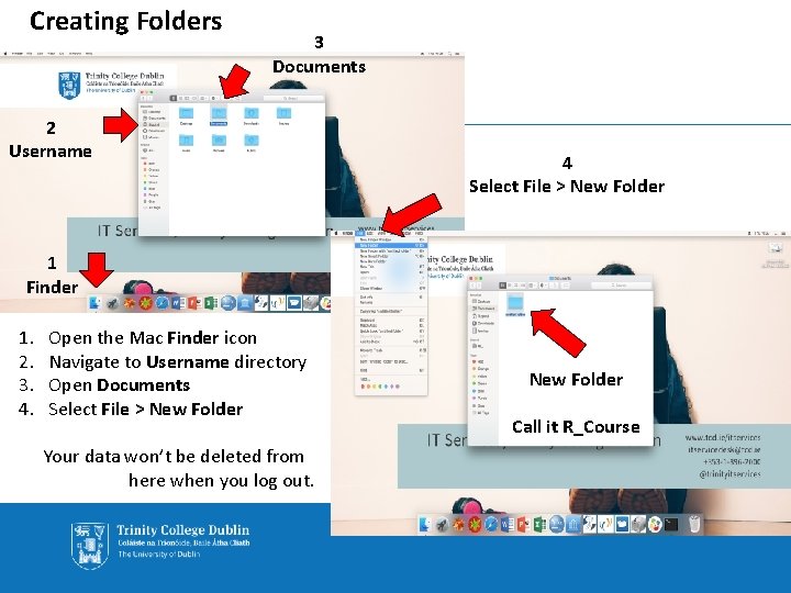
Creating Folders 3 Documents 2 Username 4 Select File > New Folder 1 Finder 1. 2. 3. 4. Open the Mac Finder icon Navigate to Username directory Open Documents Select File > New Folder Your data won’t be deleted from here when you log out. New Folder Call it R_Course

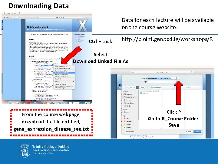
Downloading Data for each lecture will be available on the course website. Ctrl + click http: //bioinf. gen. tcd. ie/workshops/R Select Download Linked File As From the course webpage, download the file entitled, gene_expression_disease_sex. txt Click ^ Go to R_Course Folder Save

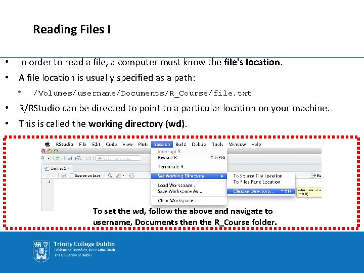
Reading Files I • In order to read a file, a computer must know the file's location. • A file location is usually specified as a path: • /Volumes/username/Documents/R_Course/file. txt • R/RStudio can be directed to point to a particular location on your machine. • This is called the working directory (wd). To set the wd, follow the above and navigate to username, Documents then the R_Course folder.

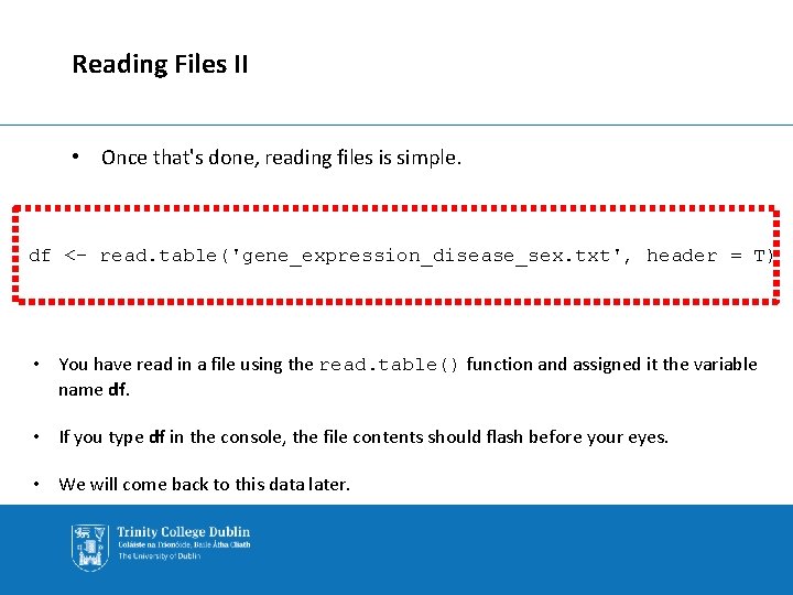
Reading Files II • Once that's done, reading files is simple. df <- read. table('gene_expression_disease_sex. txt', header = T) • You have read in a file using the read. table() function and assigned it the variable name df. • If you type df in the console, the file contents should flash before your eyes. • We will come back to this data later.

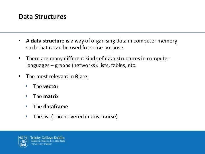
Data Structures • A data structure is a way of organising data in computer memory such that it can be used for some purpose. • There are many different kinds of data structures in computer languages – graphs (networks), lists, tables, etc. • The most relevant in R are: • The vector • The matrix • The dataframe • The list (- not covered in this course)

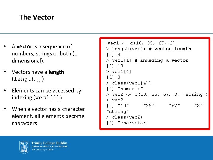
The Vector • A vector is a sequence of numbers, strings or both (1 dimensional). • Vectors have a length (length()) • Elements can be accessed by indexing (vec 1[1]) • When a vector has a character element, all elements become characters vec 1 <- c(10, 35, 67, 3) > length(vec 1) # vector length [1] 4 > vec 1[1] # indexing a vector [1] 10 > vec 1[4] [1] 3 > class(vec 1[4]) [1] "numeric" > vec 2 <- c(10, 35, 67, 3, 'string') > vec 2 [1] "10" "35" "67" "3" "string" > class(vec 2) [1] "character"

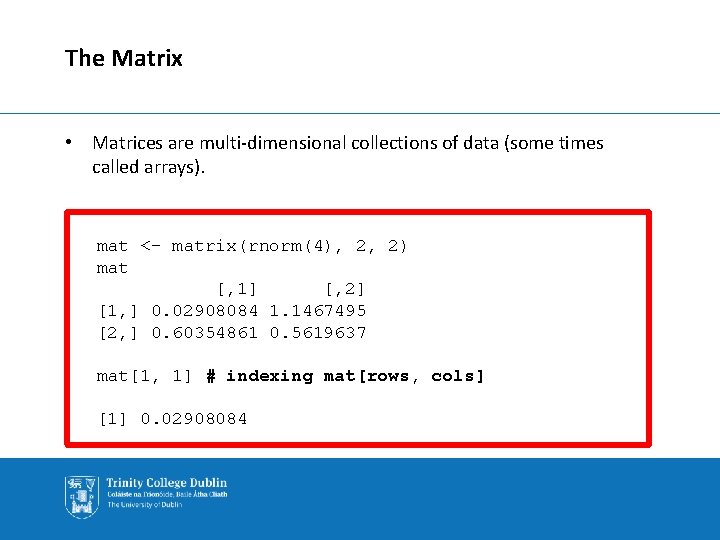
The Matrix • Matrices are multi-dimensional collections of data (some times called arrays). mat <- matrix(rnorm(4), 2, 2) mat [, 1] [, 2] [1, ] 0. 02908084 1. 1467495 [2, ] 0. 60354861 0. 5619637 mat[1, 1] # indexing mat[rows, cols] [1] 0. 02908084

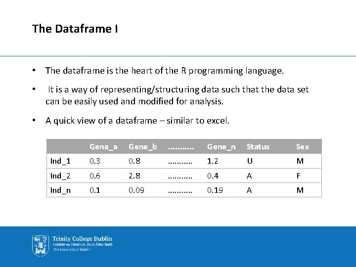
The Dataframe I • The dataframe is the heart of the R programming language. • It is a way of representing/structuring data such that the data set can be easily used and modified for analysis. • A quick view of a dataframe – similar to excel. Gene_a Gene_b . . . Gene_n Status Sex Ind_1 0. 3 0. 8 . . . 1. 2 U M Ind_2 0. 6 2. 8 . . . 0. 4 A F Ind_n 0. 1 0. 09 . . . 0. 19 A M

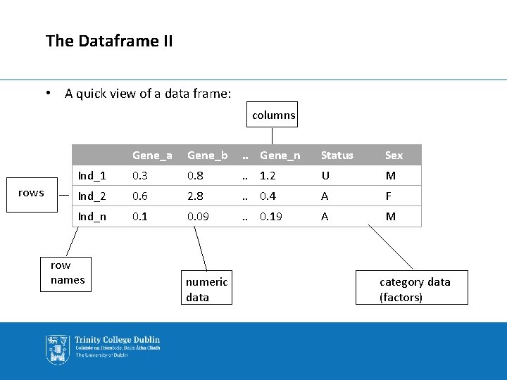
The Dataframe II • A quick view of a data frame: columns rows Gene_a Gene_b . . Gene_n Status Sex Ind_1 0. 3 0. 8 . . 1. 2 U M Ind_2 0. 6 2. 8 . . 0. 4 A F Ind_n 0. 1 0. 09 . . 0. 19 A M row names numeric data category data (factors)

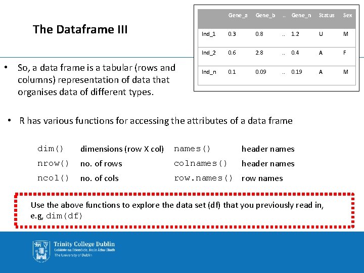
The Dataframe III • So, a data frame is a tabular (rows and columns) representation of data that organises data of different types. Gene_a Gene_b . . Gene_n Status Sex Ind_1 0. 3 0. 8 . . 1. 2 U M Ind_2 0. 6 2. 8 . . 0. 4 A F Ind_n 0. 1 0. 09 . . 0. 19 A M • R has various functions for accessing the attributes of a data frame dim() dimensions (row X col) names() header names nrow() no. of rows colnames() header names ncol() no. of cols row. names() row names Use the above functions to explore the data set (df) that you previously read in, e. g, dim(df)

The Dataframe IV > dim(df)# dimensions (rows by columns) [1] 20 12 > nrow(df) # number of rows [1] 20 > ncol(df) # number of columns [1] 12 > names(df) # header names, same as colnames(df) [1] "gene_a" "gene_b" "gene_c" "gene_d" "gene_e" "gene_f" "gene_g" "gene_h" [9] "gene_i" "gene_j" "status" "sex" > row. names(df) # row names [1] "ind_1" "ind_2" "ind_3" "ind_4" "ind_5" "ind_6" "ind_7" "ind_8" [9] "ind_9" "ind_10" "ind_11" "ind_12" "ind_13" "ind_14" "ind_15" "ind_16" [17] "ind_17" "ind_18" "ind_19" "ind_20"

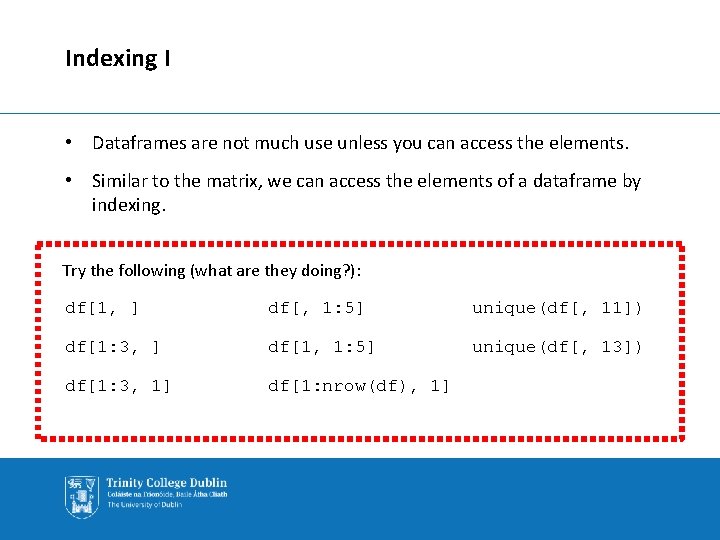
Indexing I • Dataframes are not much use unless you can access the elements. • Similar to the matrix, we can access the elements of a dataframe by indexing. Try the following (what are they doing? ): df[1, ] df[, 1: 5] unique(df[, 11]) df[1: 3, ] df[1, 1: 5] unique(df[, 13]) df[1: 3, 1] df[1: nrow(df), 1]

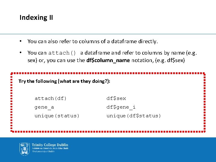
Indexing II • You can also refer to columns of a dataframe directly. • You can attach() a dataframe and refer to columns by name (e. g. sex) or, you can use the df$column_name notation, (e. g. df$sex) Try the following (what are they doing? ): attach(df) df$sex gene_a df$gene_i unique(status) unique(df$status)

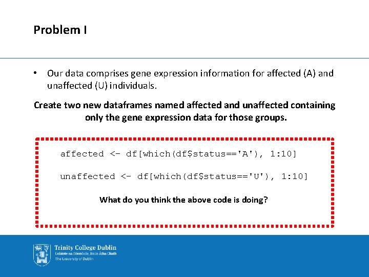
Problem I • Our data comprises gene expression information for affected (A) and unaffected (U) individuals. Create two new dataframes named affected and unaffected containing only the gene expression data for those groups. affected <- df[which(df$status=='A'), 1: 10] unaffected <- df[which(df$status=='U'), 1: 10] What do you think the above code is doing?

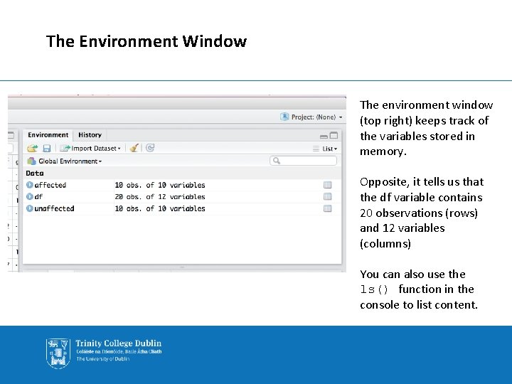
The Environment Window The environment window (top right) keeps track of the variables stored in memory. Opposite, it tells us that the df variable contains 20 observations (rows) and 12 variables (columns) You can also use the ls() function in the console to list content.

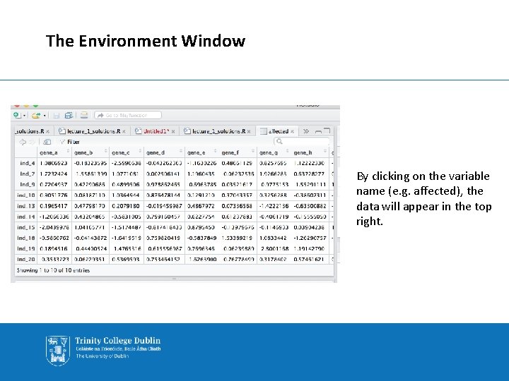
The Environment Window By clicking on the variable name (e. g. affected), the data will appear in the top right.

The History Window • The history window keeps a record of execute commands. • You can highlight code, click "to source" and the code will appear in your Rscript.

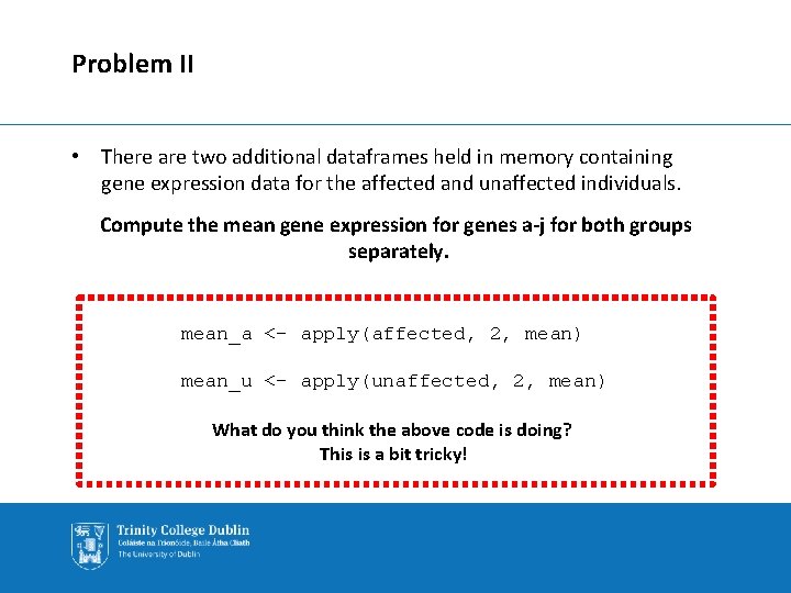
Problem II • There are two additional dataframes held in memory containing gene expression data for the affected and unaffected individuals. Compute the mean gene expression for genes a-j for both groups separately. mean_a <- apply(affected, 2, mean) mean_u <- apply(unaffected, 2, mean) What do you think the above code is doing? This is a bit tricky!

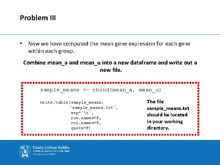
Problem III • Now we have computed the mean gene expression for each gene within each group. Combine mean_a and mean_u into a new dataframe and write out a new file. sample_means <- rbind(mean_a, mean_u) write. table(sample_means, 'sample_means. txt', sep='t', row. names=T, col. names=T, quote=F) The file sample_means. txt should be located in your working directory.

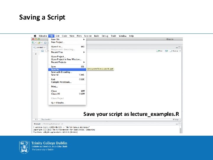
Saving a Script Save your script as lecture_examples. R

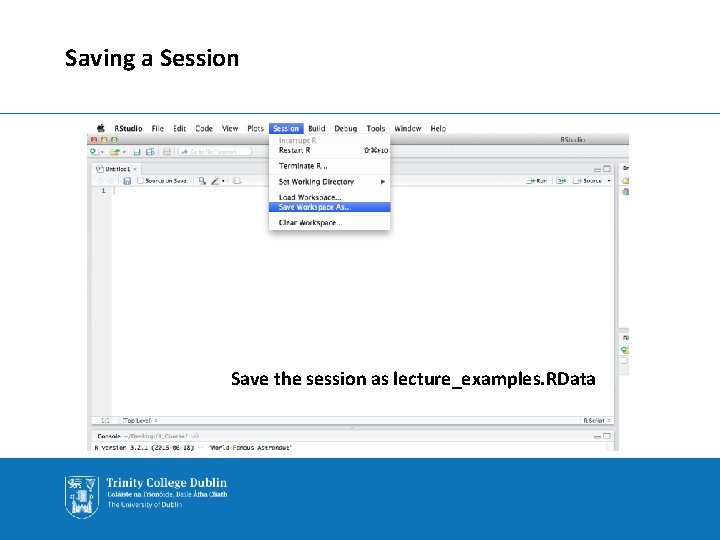
Saving a Session Save the session as lecture_examples. RData

Summary • Today we covered a lot: • R studio, variables, operators, data types, data structures, inbuilt functions • We came across a few inbuilt functions in R (the unintuitive ones are worth looking up in the help pages!) • read. table(), which(), apply(), rbind(), write. table() • Tomorrow, we will look at more advanced aspects of R syntax and basic plotting.

Lecture 1 – problem sheet • A problem sheet entitled lecture_1_problems. pdf is located on the course website (http: //bioinf. gen. tcd. ie/workshops/R). • All the code required for the problem sheet has been covered in this lecture. • Please attempt the problems for the next 30 -45 mins. • We will be on hand to help out. • Solutions will be posted this afternoon.

Thank You