Statistical Programming Using the R Language Lecture 2

Statistical Programming Using the R Language Lecture 2 Basic Concepts II Darren J. Fitzpatrick, Ph. D June 2017

Lecture I - Recap Yesterday: • Basic usage of RStudio • Some programming concepts • Variables, Data Types, Data Structures, et. c • Basic R syntax • Dealing with data frames – indexing • Reading and Writing Files

Lecture 2 - Overview • Loops & Conditionals • the WHILE loop • the FOR loop • the if(){} statemnt • Plotting • Packages • installing, loading Trinity College Dublin, The University of Dublin

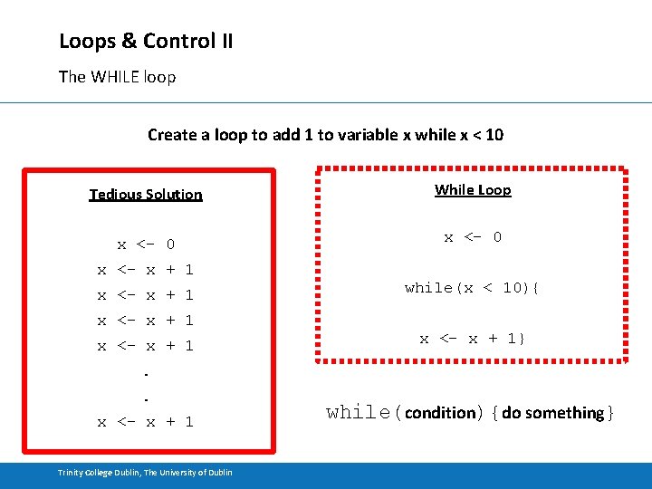
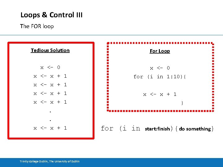
Loops & Control I • Programming often deals with repetitive tasks. • We could code these tasks repetitively or encapsulate them in a loop – one piece of code does the same task a predetermined number of times. • Loops - constructs that allow the automation of repetitive tasks without repeating the writing of code. • Iteration – each pass through a loop. • Control – the creation of a condition that determines the termination of a loop. Trinity College Dublin, The University of Dublin

Loops & Control II The WHILE loop Create a loop to add 1 to variable x while x < 10 Tedious Solution While Loop x <- 0 x <- x + 1 while(x < 10){ x <- x + 1} . . x <- x + 1 Trinity College Dublin, The University of Dublin while(condition){do something}

Loops & Control III The FOR loop Tedious Solution For Loop x <- 0 x <- x + 1 for (i in 1: 10){ x <- x + 1 } . . x <- x + 1 Trinity College Dublin, The University of Dublin for (i in start: finish){do something}

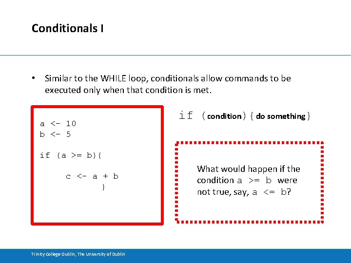
Conditionals I • Similar to the WHILE loop, conditionals allow commands to be executed only when that condition is met. a <- 10 b <- 5 if (condition){do something} if (a >= b){ c <- a + b } Trinity College Dublin, The University of Dublin What would happen if the condition a >= b were not true, say, a <= b?

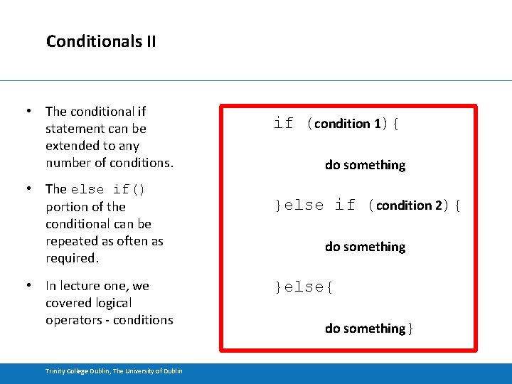
Conditionals II • The conditional if statement can be extended to any number of conditions. • The else if() portion of the conditional can be repeated as often as required. • In lecture one, we covered logical operators - conditions Trinity College Dublin, The University of Dublin if (condition 1){ do something }else if (condition 2){ do something }else{ do something}

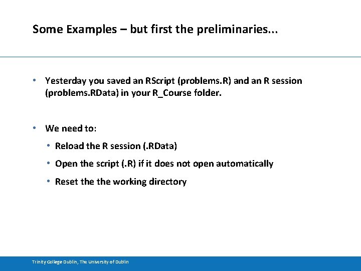
Some Examples – but first the preliminaries. . . • Yesterday you saved an RScript (problems. R) and an R session (problems. RData) in your R_Course folder. • We need to: • Reload the R session (. RData) • Open the script (. R) if it does not open automatically • Reset the working directory Trinity College Dublin, The University of Dublin

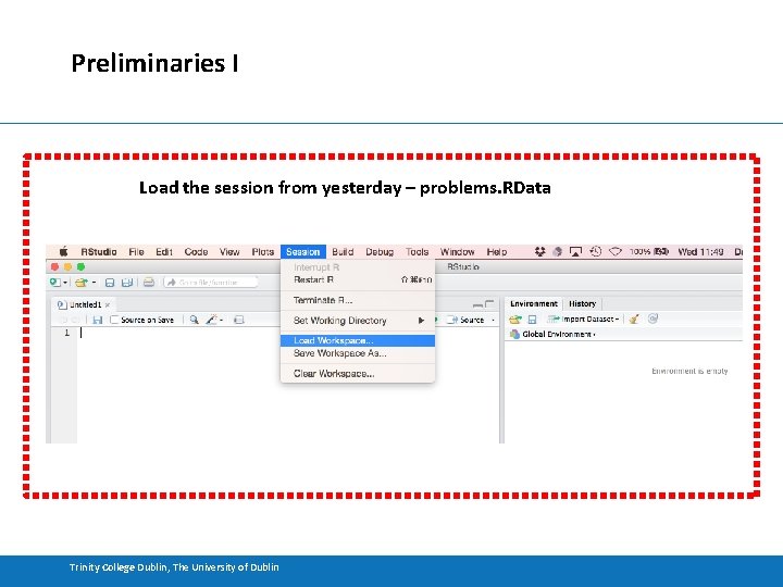
Preliminaries I Load the session from yesterday – problems. RData Trinity College Dublin, The University of Dublin

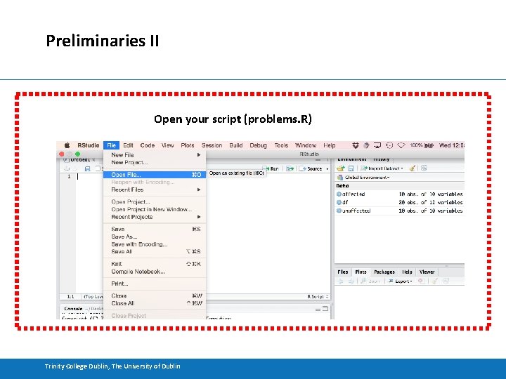
Preliminaries II Open your script (problems. R) Trinity College Dublin, The University of Dublin

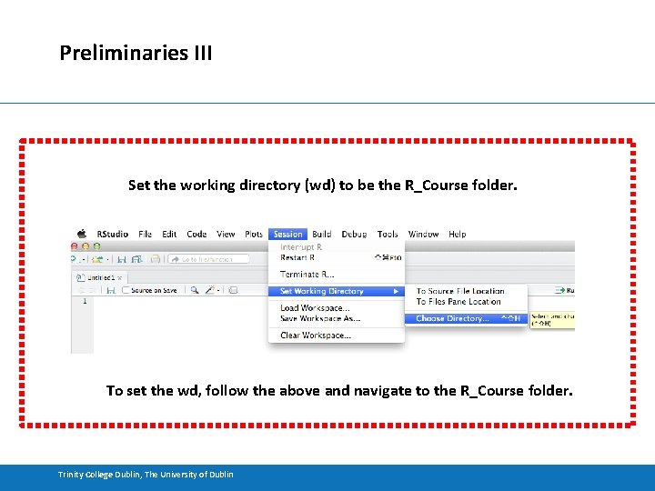
Preliminaries III Set the working directory (wd) to be the R_Course folder. To set the wd, follow the above and navigate to the R_Course folder. Trinity College Dublin, The University of Dublin

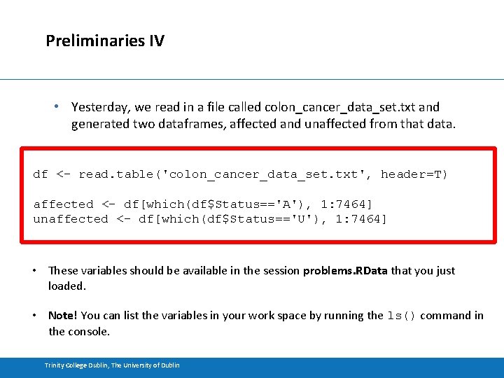
Preliminaries IV • Yesterday, we read in a file called colon_cancer_data_set. txt and generated two dataframes, affected and unaffected from that data. df <- read. table('colon_cancer_data_set. txt', header=T) affected <- df[which(df$Status=='A'), 1: 7464] unaffected <- df[which(df$Status=='U'), 1: 7464] • These variables should be available in the session problems. RData that you just loaded. • Note! You can list the variables in your work space by running the ls() command in the console. Trinity College Dublin, The University of Dublin

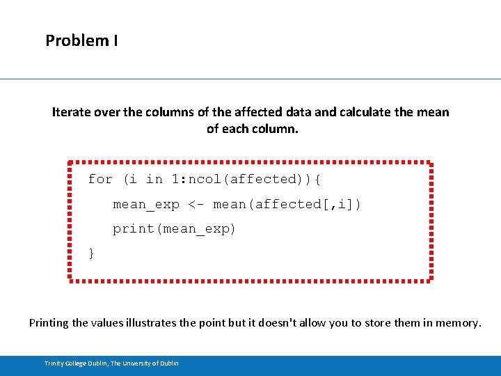
Problem I Iterate over the columns of the affected data and calculate the mean of each column. for (i in 1: ncol(affected)){ mean_exp <- mean(affected[, i]) print(mean_exp) } Printing the values illustrates the point but it doesn't allow you to store them in memory. Trinity College Dublin, The University of Dublin

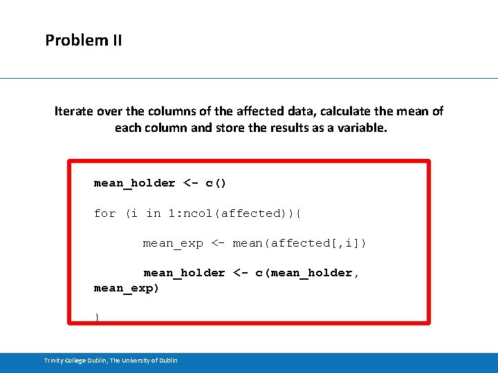
Problem II Iterate over the columns of the affected data, calculate the mean of each column and store the results as a variable. mean_holder <- c() for (i in 1: ncol(affected)){ mean_exp <- mean(affected[, i]) mean_holder <- c(mean_holder, mean_exp) } Trinity College Dublin, The University of Dublin

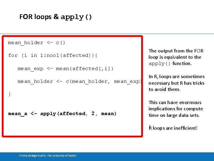
FOR loops & apply() mean_holder <- c() for (i in 1: ncol(affected)){ mean_exp <- mean(affected[, i]) mean_holder <- c(mean_holder, mean_exp) } mean_a <- apply(affected, 2, mean) The output from the FOR loop is equivalent to the apply() function. In R, loops are sometimes necessary but R has tricks to avoid them. This can have enormous implications for compute time on large data sets. } R loops are inefficient! Trinity College Dublin, The University of Dublin

Basic Plotting • R is suitable for making publication quality graphics. • R can generally create simple plots using a single function. • We will look at the following plots: • histograms (hist()) • boxplots (boxplot()) • scatterplots (plot(), scatterplot()) Trinity College Dublin, The University of Dublin

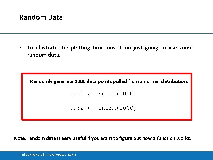
Random Data • To illustrate the plotting functions, I am just going to use some random data. Randomly generate 1000 data points pulled from a normal distribution. var 1 <- rnorm(1000) var 2 <- rnorm(1000) Note, random data is very useful if you want to figure out how a function works. Trinity College Dublin, The University of Dublin

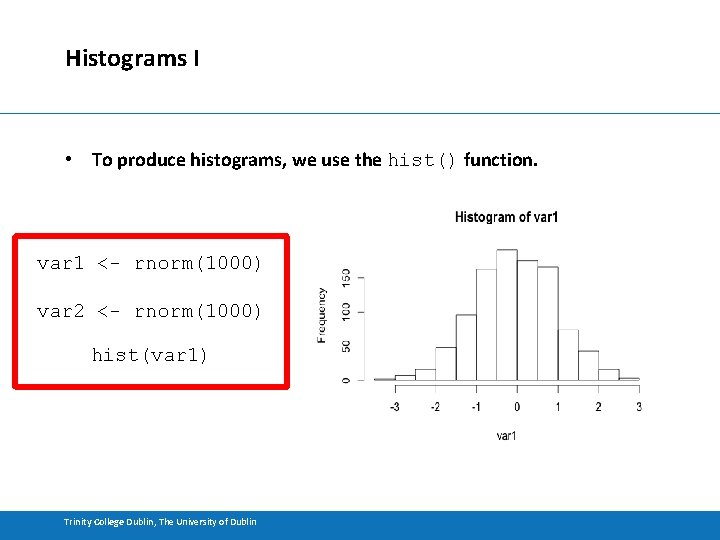
Histograms I • To produce histograms, we use the hist() function. var 1 <- rnorm(1000) var 2 <- rnorm(1000) hist(var 1) Trinity College Dublin, The University of Dublin

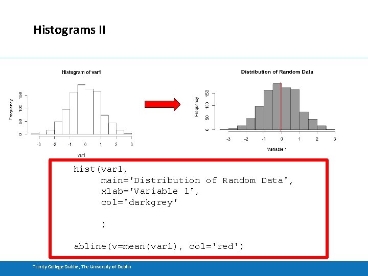
Histograms II hist(var 1, main='Distribution of Random Data', xlab='Variable 1', col='darkgrey' ) abline(v=mean(var 1), col='red') Trinity College Dublin, The University of Dublin

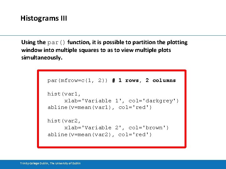
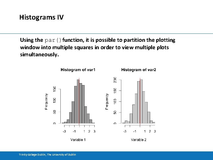
Histograms III Using the par() function, it is possible to partition the plotting window into multiple squares to as to view multiple plots simultaneously. par(mfrow=c(1, 2)) # 1 rows, 2 columns hist(var 1, xlab='Variable 1', col='darkgrey') abline(v=mean(var 1), col='red') hist(var 2, xlab='Variable 2', col='brown') abline(v=mean(var 2), col='red') Trinity College Dublin, The University of Dublin

Histograms IV Using the par()function, it is possible to partition the plotting window into multiple squares in order to view multiple plots simultaneously. Trinity College Dublin, The University of Dublin

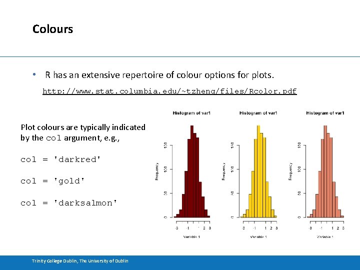
Colours • R has an extensive repertoire of colour options for plots. http: //www. stat. columbia. edu/~tzheng/files/Rcolor. pdf Plot colours are typically indicated by the col argument, e. g. , col = 'darkred' col = 'gold' col = 'darksalmon' Trinity College Dublin, The University of Dublin

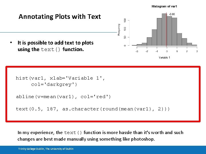
Annotating Plots with Text • It is possible to add text to plots using the text() function. hist(var 1, xlab='Variable 1', col='darkgrey') abline(v=mean(var 1), col='red') text(0. 5, 187, as. character(round(mean(var 1), 2))) In my experience, the text() function is more hassle than it's worth and such changes are best made manually using something like photoshop. Trinity College Dublin, The University of Dublin

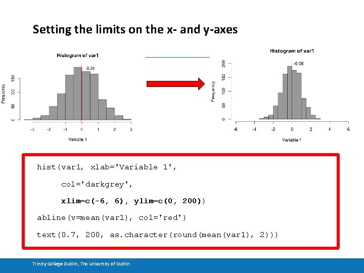
Setting the limits on the x- and y-axes hist(var 1, xlab='Variable 1', col='darkgrey', xlim=c(-6, 6), ylim=c(0, 200)) abline(v=mean(var 1), col='red') text(0. 7, 200, as. character(round(mean(var 1), 2))) Trinity College Dublin, The University of Dublin

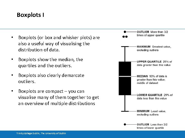
Boxplots I • Boxplots (or box and whisker plots) are also a useful way of visualising the distribution of data. • Boxplots show the median, the quartiles and the outliers. • Boxplots also clearly demarcate outliers. • Boxplots are compact – you can visualise many of them together to get an overview of multiple distributions Trinity College Dublin, The University of Dublin

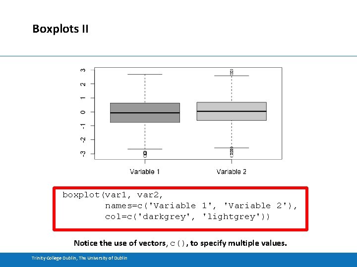
Boxplots II boxplot(var 1, var 2, names=c('Variable 1', 'Variable 2'), col=c('darkgrey', 'lightgrey')) Notice the use of vectors, c(), to specify multiple values. Trinity College Dublin, The University of Dublin

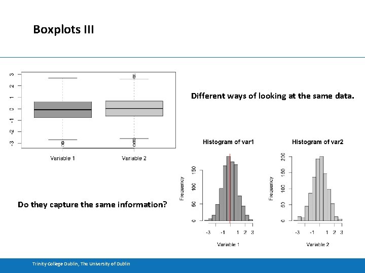
Boxplots III Different ways of looking at the same data. Do they capture the same information? Trinity College Dublin, The University of Dublin

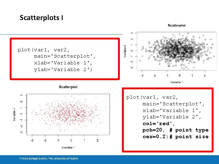
Scatterplots I plot(var 1, var 2, main='Scatterplot', xlab='Variable 1', ylab='Variable 2') plot(var 1, var 2, main='Scatterplot', xlab='Variable 1', ylab='Variable 2', col='red', pch=20, # point type cex=0. 2)# point size Trinity College Dublin, The University of Dublin

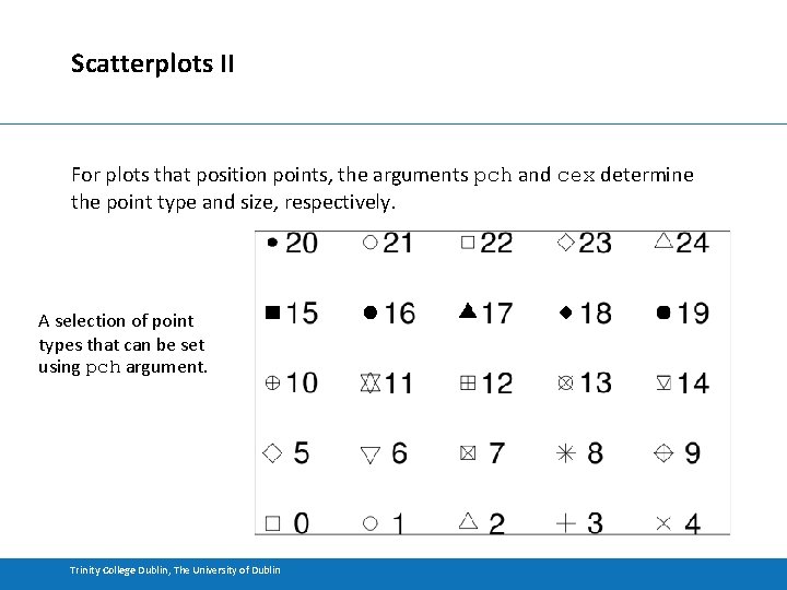
Scatterplots II For plots that position points, the arguments pch and cex determine the point type and size, respectively. A selection of point types that can be set using pch argument. Trinity College Dublin, The University of Dublin

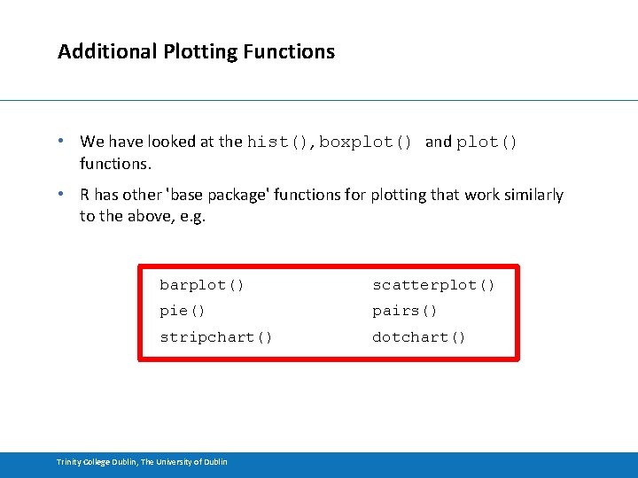
Additional Plotting Functions • We have looked at the hist(), boxplot() and plot() functions. • R has other 'base package' functions for plotting that work similarly to the above, e. g. barplot() scatterplot() pie() pairs() stripchart() dotchart() Trinity College Dublin, The University of Dublin

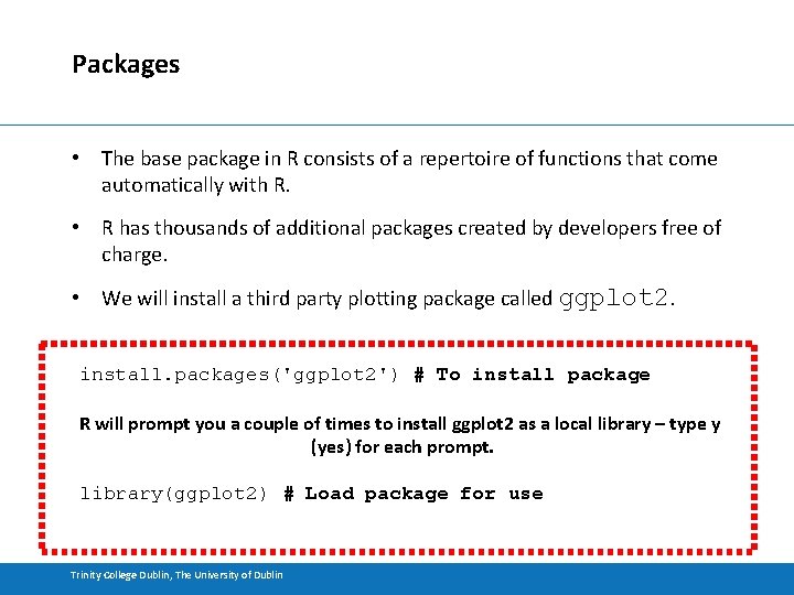
Packages • The base package in R consists of a repertoire of functions that come automatically with R. • R has thousands of additional packages created by developers free of charge. • We will install a third party plotting package called ggplot 2. install. packages('ggplot 2') # To install package R will prompt you a couple of times to install ggplot 2 as a local library – type y (yes) for each prompt. library(ggplot 2) # Load package for use Trinity College Dublin, The University of Dublin

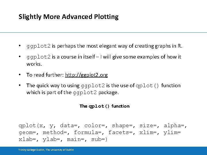
Slightly More Advanced Plotting • ggplot 2 is perhaps the most elegant way of creating graphs in R. • ggplot 2 is a course in itself – I will give some examples of how it works. • To read further: http: //ggplot 2. org • The quick way to using ggplot 2 is the use of qplot() function which is part of the ggplot 2 package. The qplot() function qplot(x, y, data=, color=, shape=, size=, alpha=, geom=, method=, formula=, facets=, xlim=, ylim= xlab=, ylab=, main=, sub=) Trinity College Dublin, The University of Dublin

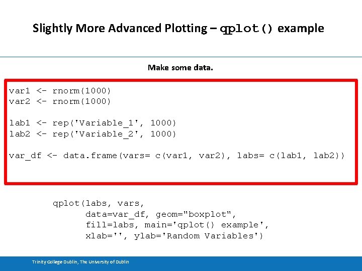
Slightly More Advanced Plotting – qplot() example Make some data. var 1 <- rnorm(1000) var 2 <- rnorm(1000) lab 1 <- rep('Variable_1', 1000) lab 2 <- rep('Variable_2', 1000) var_df <- data. frame(vars= c(var 1, var 2), labs= c(lab 1, lab 2)) qplot(labs, vars, data=var_df, geom="boxplot", fill=labs, main='qplot() example', xlab='', ylab='Random Variables') Trinity College Dublin, The University of Dublin

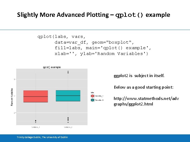
Slightly More Advanced Plotting – qplot() example qplot(labs, vars, data=var_df, geom="boxplot", fill=labs, main='qplot() example', xlab='', ylab='Random Variables') ggplot 2 is subject in itself. Below as a good starting point: http: //www. statmethods. net/adv graphs/ggplot 2. html Trinity College Dublin, The University of Dublin

Lecture 2 – problem sheet • A problem sheet entitled lecture_2_problems. pdf is located on the course website (http: //bioinf. gen. tcd. ie/workshops/R). • Some of the code required for the problem sheet has been covered in this lecture. Consult the help pages if unsure how to use a function. • Please attempt the problems for the next 30 -45 mins. • We will be on hand to help out. • Solutions will be posted this afternoon.

Thank You