Foundations of Statistic Natural Language Processing CHAPTER 6

Foundations of Statistic Natural Language Processing CHAPTER 6. STATISTICAL INFERENCE : N-GRAM MODEL OVER SPARSE DATA 1 Pusan national university 2014. 4. 22 Myoungjin, Jung

INTRODUCTION Object of Statistical NLP � Do statistical inference for the field of natural language. Statistical inference (크게 두 가지 과정으로 나눔) � 1. Taking some data generated by unknown probability distribution. ( � 2. Making some inferences about this distribution. 말뭉치 필요) (해당 말뭉치로 확률분포 추론) Divides the problem into three areas : (통계적 언어처리의 3가지 과정) � � � 1. Dividing the training data into equivalence class. 2. Finding a good statistical estimator for each equivalence class. 3. Combining multiple estimators. 2

BINS : FORMING EQUIVALENCE CLASSES Reliability vs Discrimination Ex)“large green ______” tree? mountain? frog? car? “swallowed the large green ____” pill? broccoli? � smaller n: more instances in training data, better statistical estimates (more reliability) � larger n: more information about the context of the specific instance (greater discrimination) 3

BINS : FORMING EQUIVALENCE CLASSES N-gram models “n-gram” = sequence of n words � predicting the next word : � Markov assumption Only the prior local context - the last few words – affects the next word. � Selecting an n : Vocabulary size = 20, 000 words � n Number of bins 2 (bigrams) 400, 000 3 (trigrams) 8, 000, 000 4 (4 -grams) 1. 6 x 1017 4

BINS : FORMING EQUIVALENCE CLASSES Probability dist. : P(s) where s : sentence Ex. P(If you’re going to San Francisco, be sure ……) = P(If) * P(you’re|If) * P(going|If you’re) * P(to|If you’re going) * …… Markov assumption � Only the last n-1 words are relevant for a prediction Ex. With n=5 P(sure|If you’re going to San Francisco, be) = P(sure|San Francisco , be) 5

BINS : FORMING EQUIVALENCE CLASSES 6

BINS : FORMING EQUIVALENCE CLASSES 7

BINS : FORMING EQUIVALENCE CLASSES 8

STATISTICAL ESTIMATORS Given the observed training data. How do you develop a model (probability distribution) to predict future events? (더 좋은 확률의 추정) Probability estimate � target feature Estimating the unknown probability distribution of n-grams. 9

STATISTICAL ESTIMATORS Notation for the statistical estimation chapter. N Number of training instances B Number of bins training instances are divided into w 1 n C(w 1…wn) r An n-gram w 1…wn in the training text Freq. of an n-gram f( • ) Freq. estimate of a model Nr Number of bins that have r training instances in them Tr Total count of n-grams of freq. r in further data h ‘History’ of preceding words 10

STATISTICAL ESTIMATORS Example - Instances in the training corpus: “inferior to ____” 11

MAXIMUM LIKELIHOOD ESTIMATION (MLE) Definition � Using the relative frequency as a probability estimate. Example : � In corpus, found 10 training instances of the word “comes across” � 8 times they were followed by “as” : P(as) = 0. 8 � Once by “more” and “a” : P(more) = 0. 1 , P(a) = 0. 1 � Not among the above 3 word : P(x) = 0. 0 Formula 12

MAXIMUM LIKELIHOOD ESTIMATION (MLE) 13

MAXIMUM LIKELIHOOD ESTIMATION (MLE) Example 1. A Paragraph Using Training Data The bigram model uses the preceding word to help predict the next word. (End) In general, this helps enormously, and gives us a much better model. (End) In some cases the estimated probability of the word that actually comes next has gone up by about an order of magnitude (was, to, sisters). (End) However, note that the bigram model is not guaranteed to increase the probability estimate. (End) C(the)=7 C(bigram)=2 C(model)=3 C(the, bigram)=2 C(the, bigram, model)=2 14

LAPLACE’S LAW, LIDSTONE’S LAW AND THE JEFFREYS-PERKS LAW Laplace’s law(1814; 1995) � Add a little bit of probability space to unseen events 15

LAPLACE’S LAW, LIDSTONE’S LAW AND THE JEFFREYS-PERKS LAW Word (N=79 : B=seen(51)+unseen(70)=121) MLE Laplace’s law 0. 0886076 0. 0400000 0. 2857143 0. 0050951 1. 0000000 0. 0083089 16

LAPLACE’S LAW, LIDSTONE’S LAW AND THE JEFFREYS-PERKS LAW Page 202 -203 (Associated Press[AP] newswire yielded a vocabulary) unseen event에 대한 약간의 확률 공간을 추가 but 너무 많은 공간을 추가하였다. 44 milion의 경우 voca 400653 발생 -> 160, 000, 000 bigram 발생 Bins의 개수가 training instance보다 많아지게 되는 문제가 발생 • Lap law는 unseen event에 대한 확률공간을 위해 분모에 B를 삽입 하였지만 결과적으로 약 46. 5%의 확률공간을 unseen event에 주게 되었다. • N 0 * P lap(. ) = 74. 671, 100, 000 * 0, 000137/22, 000 = 0. 465 17

LAPLACE’S LAW, LIDSTONE’S LAW AND THE JEFFREYS-PERKS LAW Lidstone’s law(1920) and the Jeffreys-Perks law(1973) � Lidstone’s Law add some positive value � Jeffreys-Perks Law = 0. 5 Called ELE (Expected Likelihood Estimation) 18

LIDSTONE’S LAW Using Lidstone’s law, instead of adding one, add some smaller value , where the parameter is in the range . And . 19

LIDSTONE’S LAW Here, gives the maximum likelihood estimate, gives the Laplace’s law, if tends to then we have the uniform estimate represents the trust we have in relative frequencies. implies more trust in relative frequencies than the Laplace's law while represents less trust in relative frequencies. . In practice, people use values of in the range , a common value being . (Jeffreys-Perks law) 20

JEFFREYS-PERKS LAW Using Lidstone’s law, MLE ( Lidstone’s law ) ( ) Jeffreys-Perks ( ) Lidstone’s law ( Laplace’s law Lidstone’s law ) ( ) A 0. 0886 0. 0633 0. 0538 0. 0470 0. 0400 0. 0280 B 0. 2857 0. 0081 0. 0063 0. 0056 0. 0051 0. 0049 C 1. 0000 0. 0084 0. 0085 0. 0083 *A: , B: , C: 21

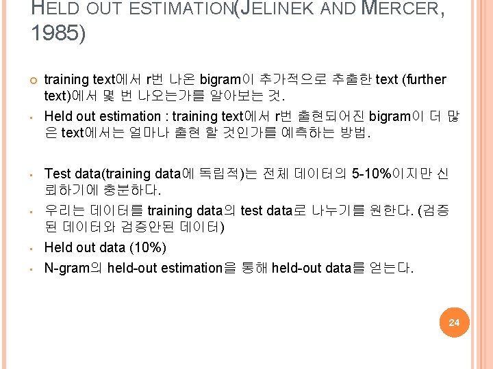
HELD OUT ESTIMATION(JELINEK AND MERCER, 1985) For each n-gram, , let : = frequency of in training data = frequency of in held out data Let be the total number of times that all n-grams that appeared r times in the training text appeared in the held out data. An estimate for the probability of one of these n-gram is : where . 22

HELD OUT ESTIMATION(JELINEK AND MERCER, 1985) [Full text ( ) : , respectively], unseen word : I don't know. [Word ( ) : , unseen word : 70, respectively] : (Training Data) [Word ( ) : , unseen word : 51 - , respectively] : (Held out Data) (1 -gram) Traing data : , ( ) Held out data : , , ( ) 23

CROSS-VALIDATION (DELETED ESTIMATION; JELINEK AND MERCER, 1985) Use data for both training and validation Ø Divide test data into 2 parts § Train on A, validate on B § Train on B, validate on A Ø Combine two models A B train validate Model 1 validate train Model 2 Model 1 + Model 2 Final Model 25

CROSS-VALIDATION (DELETED ESTIMATION; JELINEK AND MERCER, 1985) Cross validation : training data is used both as � initial training data � held out data On large training corpora, deleted estimation works better than held-out estimation 26

CROSS-VALIDATION (DELETED ESTIMATION; JELINEK AND MERCER, 1985) [Full text ( ) : , respectively], unseen word : I don't know. [Word ( ) : , unseen word : 70, respectively] : (Training Data) [A-part word ( ) : , unseen word : 101, respectively] [B-part word ( ) : , unseen word : 90 - , respectively] A-part data : , ( ) B-part data : , ( ) 27 , .

CROSS-VALIDATION (DELETED ESTIMATION; JELINEK AND MERCER, 1985) [B-part word ( ) : , unseen word : 90 - , respectively] [A-part word ( ) : , unseen word : 101+ , respectively] B-part data : , ( ) A-part data : , ( ) , . [Result] 28 , .

CROSS-VALIDATION (DELETED ESTIMATION; JELINEK AND MERCER, 1985) Held out estimation개념으로 우리가 training data를 두 부 분으로 나눔으로써 같은 효과를 얻는다. 이러한 메소드를 cross validation이라 한다. 더 효과적인 방법. 두 방법을 합치므로써 Nr 0, Nr 1의 차이 를 감소 시킨다. 큰 training curpus내의 deleted estimation은 held-out estimation보다 더 신뢰적이다. 29

GOOD-TURING ESTIMATION(GOOD, 1953) : [BINOMIAL DISTRIBUTION] (r* is an adjusted frequency) (E denotes the expectation of random variable) 30

GOOD-TURING ESTIMATION(GOOD, 1953) : [BINOMIAL DISTRIBUTION] 31

NOTE 32

NOTE 33

COMBINING ESTIMATORS 34

COMBINING ESTIMATORS 35

COMBINING ESTIMATORS 36

COMBINING ESTIMATORS 37

COMBINING ESTIMATORS 38

NOTE 39

NOTE 40

NOTE 41

NOTE 42

NOTE 43

NOTE 44

NOTE 45