SPATIAL STATISTICS ANALYSIS OF POINT PATTERNS OUTLINE ANALYSIS

SPATIAL STATISTICS ANALYSIS OF POINT PATTERNS

OUTLINE ANALYSIS OF POINT PATTERNS 1. Introduction 2. Point Pattern Descriptors § Central Tendency § Dispersion and Orientation 3. Point Pattern Analyzers § Case Studies § Visualizing Spatial Point Patterns § Exploring Spatial Point Patterns a. Quadrat Methods b. Kernel Estimation c. Nearest Neighbor Distance d. The K Function 2

Introduction This section is considered to investigate methods for analysis of a set of point locations, which is often referred as “point pattern”. A spatial point process is any stochastic ( event or system that is unpredictable because of a random variable) mechanism that generates a countable set of events (si) in a plane 3

Basic Definitions: Event: The location of observed occurrence of the spatial phenomena, differentiated from other arbitrary locations in the study region. Mapped point pattern: All relevant events in a study area R have been recorded Point: Arbitrary locations or locations other than events. Sampled point pattern: Events are recorded from a sample of different areas 4

Objectives: v To determine if there is a tendency for points to exhibit a systematic pattern (i. e. some form of regularity or clustering) v If there is a systematic pattern, then to examine at what spatial scale this pattern occurs and whether particular clusters are associated with proximity to particular sources of some factors. v To estimate how the intensity of points varies across the study region v To seek models to account/explain for observed point patterns 5

Analysis Approach: v Events may have attributes which can be used to distinguish types – but it is the location pattern that is analyzed v Patterns in event locations are the focus v Stochastic aspect is where events are likely to occur v Does a pattern exhibit clustering or regularity? v Over what spatial scales do patterns exist? 6

E. g. Such methods are relevant to the study of patterns of occurrence of: v v v Diseases Crime types Earthquake epicenters Plant distributions Etc. A Point pattern is simple example of spatial data, since the data contains only the coordinates of events. However, this does not mean that the analysis is any easier than for other spatial data types. In fact from a statistical perspective, point patterns can in some ways be mathematically more complex to handle. 7

Usually data in point pattern analysis comprise: 1. Locations (coordinates) 1. Attributes (tree types, crime type, date of disease notification, etc. ) A point pattern is a data set consisting of a series of point locations (s 1, s 2, …) in some study region R at which events of interest have occurred. 8

Basic Assumptions: 1. Data present a complete set of events in the study region R, which is called mapped point pattern. i. e. all relevant events occurred in R have been recorded. !!!Remark: Some point pattern analysis are directed towards extracting limited information about a point process, by recording events in a sample of different areas of the whole region, which is called sampled point pattern. E. g. Field studies in forestry, ecology or biology, where complete enumeration is not feasible. 9

Basic Assumptions: 2. The study region R might be of any arbitrary shape. Some of the methods can be applied to only regions, which are square or rectangle. 3. In order to eliminate edge effects, a suitable guard area between perimeter of the original study region and sub-region within which analysis is performed is left. 4. In all cases, the final area selected for study is assumed to be in some sense representative of any larger region from which it has been selected. 10

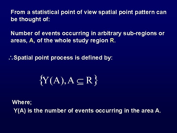
From a statistical point of view spatial point pattern can be thought of: Number of events occurring in arbitrary sub-regions or areas, A, of the whole study region R. Spatial point process is defined by: Where; Y(A) is the number of events occurring in the area A.

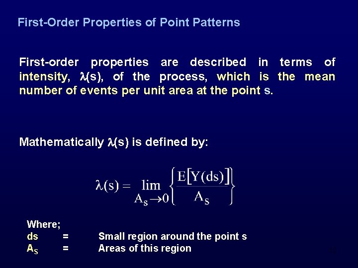
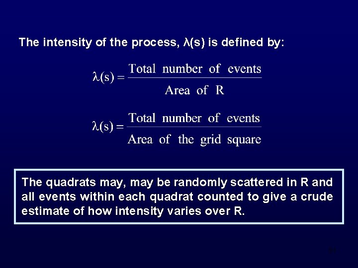
First-Order Properties of Point Patterns First-order properties are described in terms of intensity, (s), of the process, which is the mean number of events per unit area at the point s. Mathematically (s) is defined by: Where; ds = AS = Small region around the point s Areas of this region 12

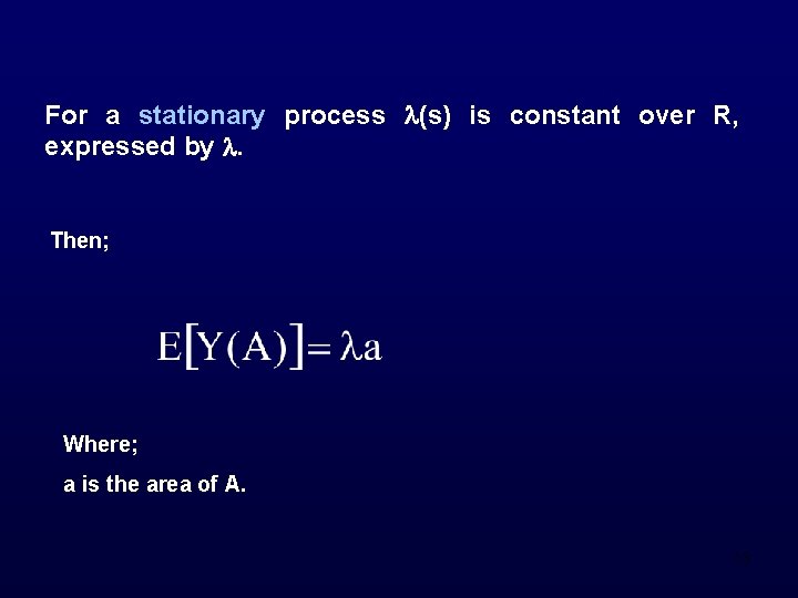
For a stationary process (s) is constant over R, expressed by . Then; Where; a is the area of A. 13

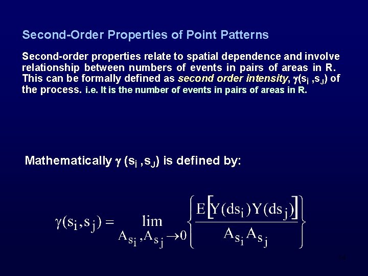
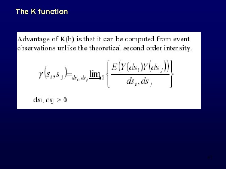
Second-Order Properties of Point Patterns Second-order properties relate to spatial dependence and involve relationship between numbers of events in pairs of areas in R. This can be formally defined as second order intensity, (sİ , s. J) of the process. i. e. It is the number of events in pairs of areas in R. Mathematically (sİ , s. J) is defined by: 14

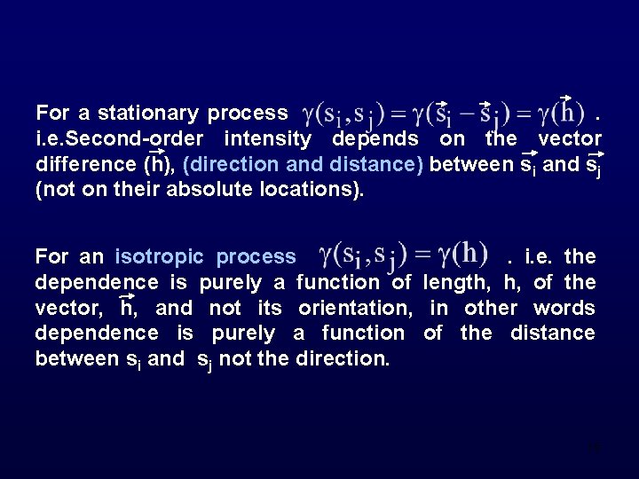
For a stationary process. i. e. Second-order intensity depends on the vector difference (h), (direction and distance) between si and sj (not on their absolute locations). For an isotropic process. i. e. the dependence is purely a function of length, h, of the vector, h, and not its orientation, in other words dependence is purely a function of the distance between si and sj not the direction. 15

POINT PATTERN DESCRIPTORS 16

The Nature of Point Features Point pattern descriptors cover: § The methods for determining the overall patterns of a given set of points. § Measures used to describe the magnitude of spatial dispersion of a given set of points. § How the direction bias of a set of points can be extracted statistically. 17

Central Tendency of Point Distributions § A set of point descriptors provide certain descriptive information on the distribution of a set of points. § Central tendency information, mean centres, weighted mean centres, and median centres provide a good summary of how a set of points distributes in the geographic space. § To describe the spatial dispersion characteristics of a set of points, the measures of standard distance and standard ellipse will be discussed. These measures indicate the spatial variation and orientation of a point distribution. 18

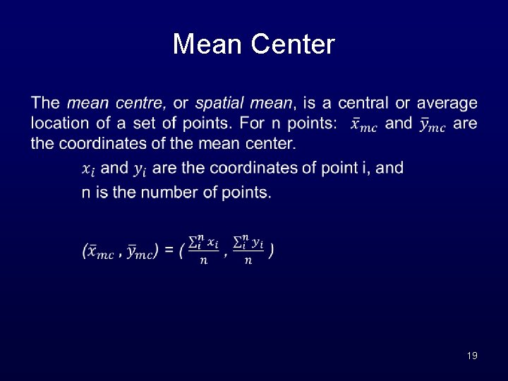
Mean Center • 19

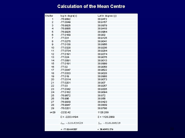
Calculation of the Mean Centre Shelter 1 2 3 4 5 6 7 8 9 10 11 12 13 14 15 16 17 18 19 20 21 22 23 24 25 26 27 28 29 n=29 log in degre(x) -76. 9892 -77. 0049 -76. 9926 -76. 9886 -76. 9926 -77. 0189 -77. 031 -77. 0275 -77. 0138 -77. 0328 -77. 0734 -77. 0191 -77. 024 -77. 0091 -77. 0191 -77. 02 -77. 0047 -77. 0333 -77. 019 -77. 0314 -77. 0201 -77. 0342 -77. 0182 -76. 9672 -76. 996 -76. 9939 -76. 9947 -76. 0201 Lat in degree (y) 38. 9472 38. 9157 38. 8979 38. 9418 38. 8964 38. 902 38. 9125 38. 9041 38. 8956 38. 9206 38. 9284 38. 9374 38. 9076 38. 9013 38. 8999 38. 9058 38. 9622 38. 9028 38. 8988 38. 9073 38. 907 38. 9257 38. 9305 38. 9094 38. 872 38. 856 38. 8423 38. 8809 38. 8798 -2232. 42 1128. 289 Σ = -2233. 4194 Σ = 1128. 2889 = -77. 01446207 = 38. 90651379 20

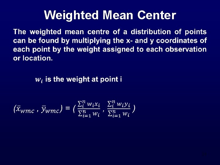
Weighted Mean Center • 21

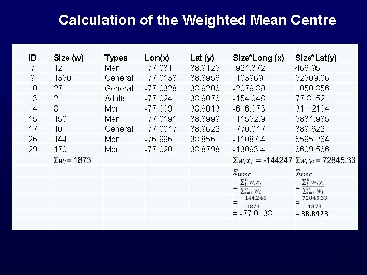
Calculation of the Weighted Mean Centre ID 7 9 10 13 14 15 17 26 29 Size (w) 12 1350 27 2 8 150 10 144 170 Types Men General Adults Men General Men Lon(x) -77. 031 -77. 0138 -77. 0328 -77. 024 -77. 0091 -77. 0191 -77. 0047 -76. 996 -77. 0201 Lat (y) 38. 9125 38. 8956 38. 9206 38. 9076 38. 9013 38. 8999 38. 9622 38. 856 38. 8798 Size*Long (x) -924. 372 -103969 -2079. 89 -154. 048 -616. 073 -11552. 9 -770. 047 -11087. 4 -13093. 4 Size*Lat(y) 466. 95 52509. 06 1050. 856 77. 8152 311. 2104 5834. 985 389. 622 5595. 264 6609. 566 = -77. 0138 = 38. 8923 22

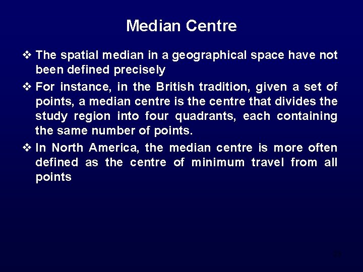
Median Centre v The spatial median in a geographical space have not been defined precisely v For instance, in the British tradition, given a set of points, a median centre is the centre that divides the study region into four quadrants, each containing the same number of points. v In North America, the median centre is more often defined as the centre of minimum travel from all points 23

Dispersion and Orientation of Point Distributions § Two sets of points may occupy the same geographic space and may be interrelated. For example, one set of points represents the location of forest fires and the other the locations of camping cabins in a wildlife region. They may have the same overall locations, buy forest fire have a more dispersed spatial pattern than cabins. § In additional to spatial central tendency, it may be interesting to evaluate the magnitude of dispersion of locations and the orientation of the spatialdistribution. 24

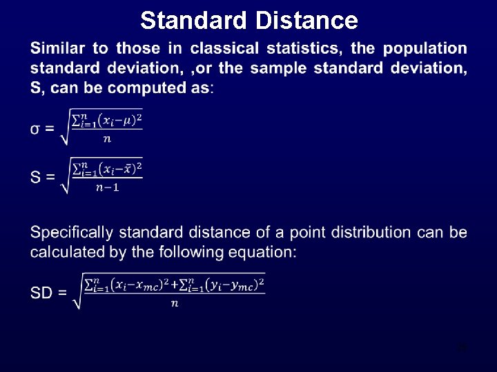
Standard Distance • 25

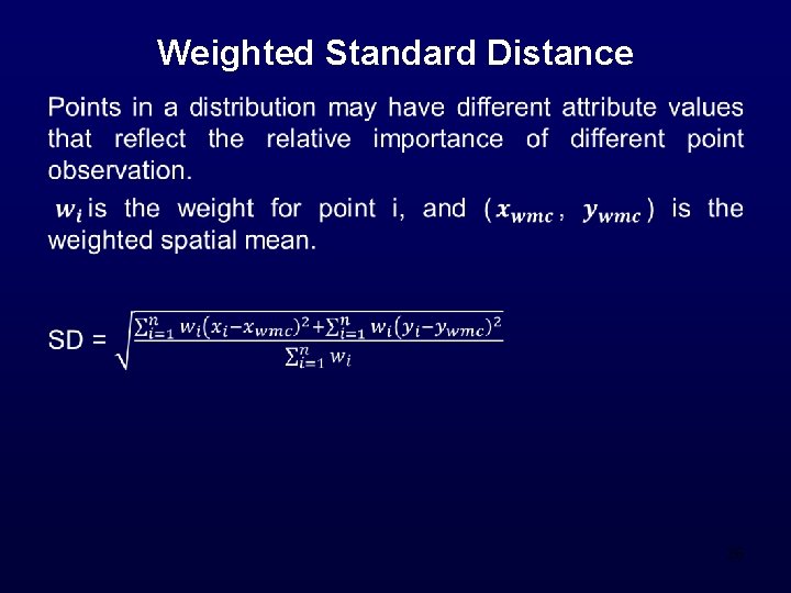
Weighted Standard Distance • 26

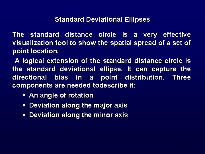
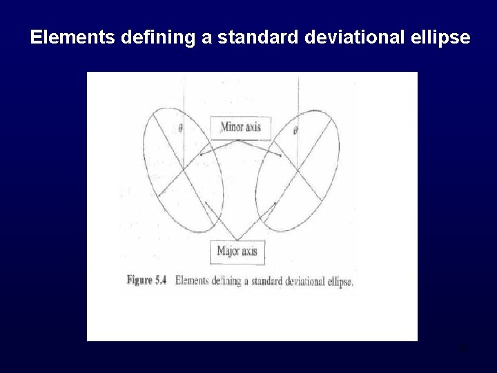
Standard Deviational Ellipses The standard distance circle is a very effective visualization tool to show the spatial spread of a set of point location. A logical extension of the standard distance circle is the standard deviational ellipse. It can capture the directional bias in a point distribution. Three components are needed todescribe it: § An angle of rotation § Deviation along the major axis § Deviation along the minor axis 27

Elements defining a standard deviational ellipse 28

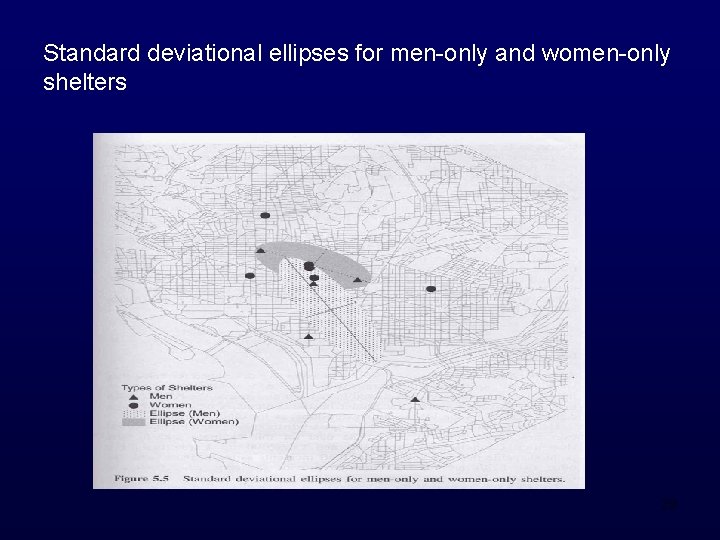
Standard deviational ellipses for men-only and women-only shelters 29

POINT PATTERN ANALYZERS 30

Case Studies The following cases will be of concern when studying point patterns. 1. The locations of craters in a volcanic field in Uganda 2. The locations of granite tors in Bodmin Moor 3. The locations of redwood seedlings in a forest 4. The locations of centers of biological cells in a section of tissue 5. The locations of the homes of juvenile offenders on a Cardiff estate 6. Locations of “theft from property” offences in Oklahoma City 7. Locations of cases of cancer larynx and lung in part of Lancashire 8. Locations of Burkitt’s lymphoma in an area of Uganda 31

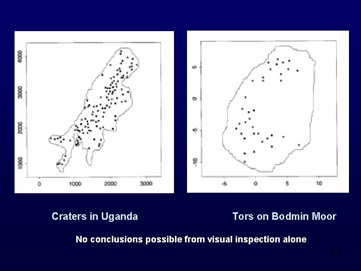
1. The locations of craters in a volcanic field in Uganda The data set involves the locations of centers of craters of 120 volcanoes in the Bunyaruguru volcanic field in west Uganda. A map of the distribution shows a broad regional trend in a north-easterly direction, representing elongation along a major fault. 32

The purposes of studying this case: v variation. v smaller scale. v To answer the following questions: Is the distribution random within the study region? Is there evidence of clustering or regularity? v To test the following hypotheses: It is expected that rift faults would guide volcanic activity to the surface, along fractures or lines of weakness. The hypothesis is to test weather this holds true. 33

2. The locations of granite tors in Bodmin Moor There are 35 locations of granite tors and on a large scale there is clear spatial patterning. The purposes of studying this case: v randomness at smaller scales. v. To find the if regularity in the distribution is valid for only small distances. To minev patterning at slightly longer distances. 34

3. The locations of redwood seedlings in a forest There are 62 redwood seedlings distributed in a square region of 23 m 2. The purposes of studying this case: some see To evidence v clustering of around existing parent trees. 35

4. The locations of centers of biological cells in a section of tissue There are centers of 42 biological cells in a section of tissue. The purposes of studying this case: v. To know whethere is evidence for departures from randomness in such data. v. To answer the following question: Are such cells clustered or regular? 36

5. The locations of the homes of juvenile offenders on a Cardiff estate The data recorded in 1971. The purposes of studying this case: v 37

6. Locations of “theft from property” offences in Oklahoma City The data are taken from research done on crime in Oklahoma City in late 1970 s and comprise two distinct categories of events. One set refers to offences committed by whites, the other by blacks. 38

The purposes of studying this case: v To see if the spatial pattern of the events differ v To investigate if the two sub-groups have different activity places v To answer the following questions: Do the crimes committed by different groups display different spatial patterns? Are those for one group clustered or aggregated in some way, while those for the other group are more random? 39

7. Locations of cases of cancer larynx and lung in part of Lancashire The data are for a part of Lancashire in U. K. and have been collected over a 10 year period 1974 -83. Lung cancer is quite a common disease and there are 917 cases in the study area. Larynx cancer rare and there are only 57 cases notified during the study period. The purposes of studying this case: v To investigate if the residents living near the site of an old industrial waste incinerator that their health had been affected by exposure to the by-products of the incineration process. 40

8. Locations of Burkitt’s lymphoma in an area of Uganda The data comprise information on 188 cases of Burkitt’s lymphoma (a cancer affecting usually the jaw and abdomen, primarily in children) in the West Nile district of Uganda for the time period of 1961 -75. The purposes of studying this case: v 41

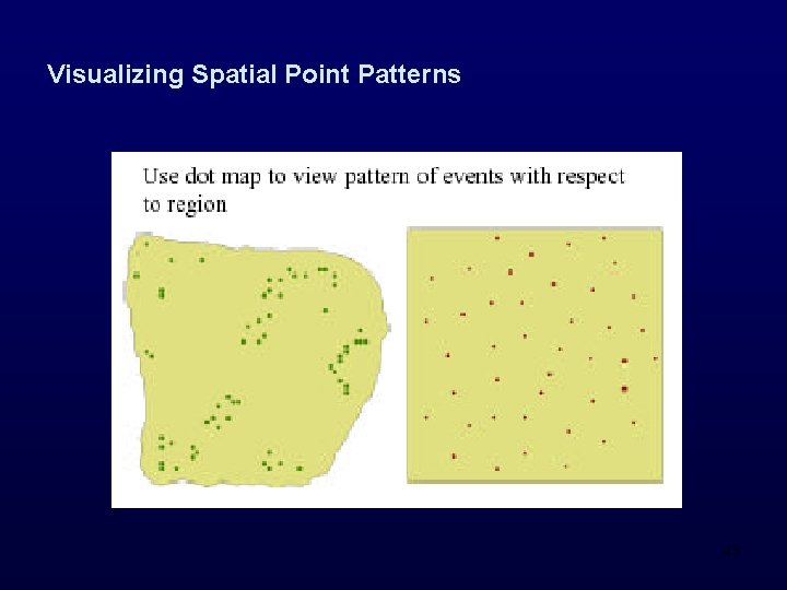
Visualizing Spatial Point Patterns Point patterns are visualized by the use of dot map. This gives an initial impression of the shape of the study region and any obvious pattern present in the distribution of events. !!!Remark: Intuitive ideas about what constitutes as “random pattern” can be misleading. Generally it is hard to come to any conclusion purely on the basis of a visual analysis. 42

Visualizing Spatial Point Patterns 43

Craters in Uganda Tors on Bodmin Moor No conclusions possible from visual inspection alone 44

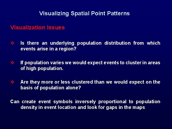
Visualizing Spatial Point Patterns Visualization Issues v Is there an underlying population distribution from which events arise in a region? v If population varies we would expect events to cluster in areas of high population. v Are they more or less clustered than we would expect on the basis of population alone? Can create event symbols inversely proportional to population density in event location and look for gaps in the maps 45

Exploring Spatial Point Patterns The methods of exploration of point patterns are divided into two: q 46

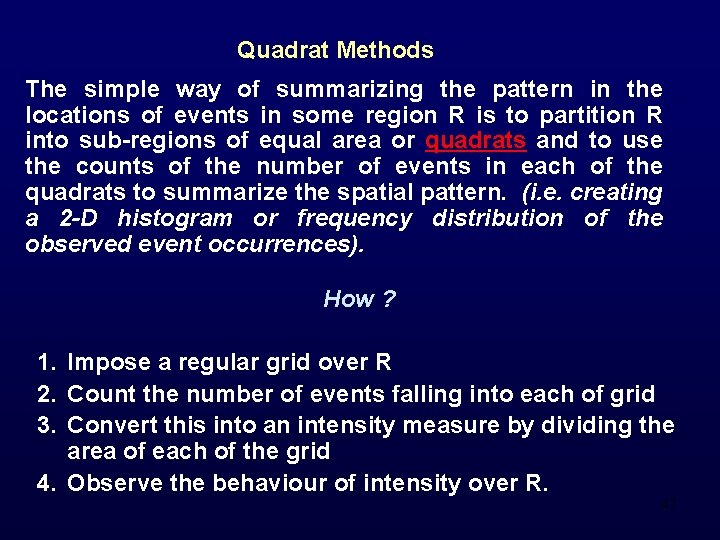
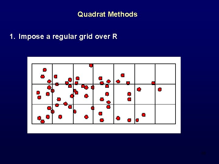
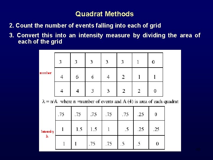
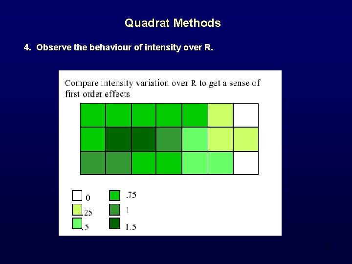
Quadrat Methods The simple way of summarizing the pattern in the locations of events in some region R is to partition R into sub-regions of equal area or quadrats and to use the counts of the number of events in each of the quadrats to summarize the spatial pattern. (i. e. creating a 2 -D histogram or frequency distribution of the observed event occurrences). How ? 1. Impose a regular grid over R 2. Count the number of events falling into each of grid 3. Convert this into an intensity measure by dividing the area of each of the grid 4. Observe the behaviour of intensity over R. 47

Quadrat Methods 1. Impose a regular grid over R 48

Quadrat Methods 2. Count the number of events falling into each of grid 3. Convert this into an intensity measure by dividing the area of each of the grid 49

Quadrat Methods 4. Observe the behaviour of intensity over R. 50

The intensity of the process, λ(s) is defined by: The quadrats may, may be randomly scattered in R and all events within each quadrat counted to give a crude estimate of how intensity varies over R. 51

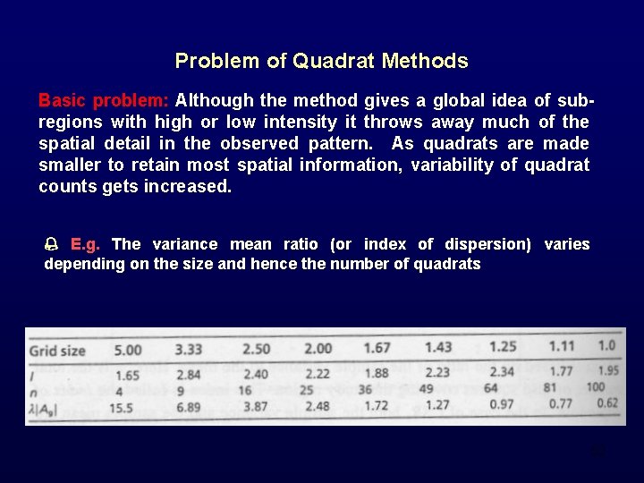
Problem of Quadrat Methods Basic problem: Although the method gives a global idea of subregions with high or low intensity it throws away much of the spatial detail in the observed pattern. As quadrats are made smaller to retain most spatial information, variability of quadrat counts gets increased. E. g. The variance mean ratio (or index of dispersion) varies depending on the size and hence the number of quadrats 52

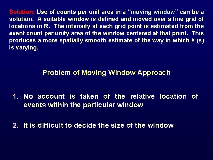
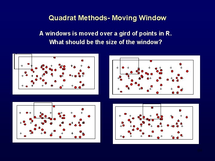
Solution: Use of counts per unit area in a “moving window” can be a solution. A suitable window is defined and moved over a fine grid of locations in R. The intensity at each grid point is estimated from the event count per unity area of the window centered at that point. This produces a more spatially smooth estimate of the way in which λ (s) is varying. Problem of Moving Window Approach 1. No account is taken of the relative location of events within the particular window 2. It is difficult to decide the size of the window 53

Quadrat Methods- Moving Window A windows is moved over a gird of points in R. What should be the size of the window? 54

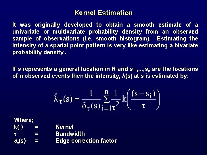
Kernel Estimation It was originally developed to obtain a smooth estimate of a univariate or multivariate probability density from an observed sample of observations (i. e. smooth histogram). Estimating the intensity of a spatial point pattern is very like estimating a bivariate probability density. If s represents a general location in R and s 1 , . . . , sn are the locations of n observed events then the intensity, λ(s) at s is estimated by: Where; k( ) = = (s) = Kernel Bandwidth Edge correction factor 55

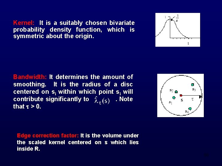
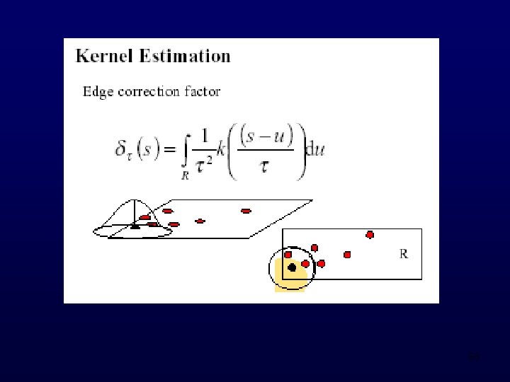
Kernel: It is a suitably chosen bivariate probability density function, which is symmetric about the origin. Bandwidth: It determines the amount of smoothing. It is the radius of a disc centered on si within which point si will contribute significantly to. Note that > 0. Edge correction factor: It is the volume under the scaled kernel centered on s which lies inside R. 56

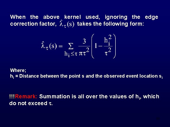
For any chosen kernel and bandwidth, values of can be estimated at locations on a suitably chosen fine grid over R to provide a useful visual indication of the variation in the intensity over the study region. Most of the time, for reasonably possible probability distributions of k ( ), the kernel estimate will be very similar for a given bandwidth . A typical choice of k ( ) might be the quadratic kernel: 57

When the above kernel used, ignoring the edge correction factor, takes the following form: Where; hi = Distance between the point s and the observed event location s i !!!Remark: Summation is all over the values of hi, which do not exceed . 58

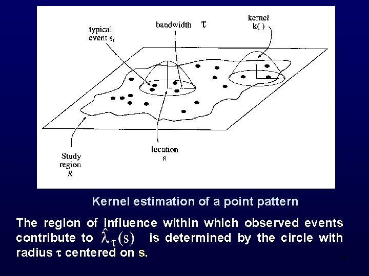
Kernel estimation of a point pattern The region of influence within which observed events contribute to is determined by the circle with radius centered on s. 59

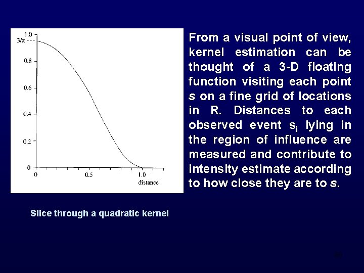
From a visual point of view, kernel estimation can be thought of a 3 -D floating function visiting each point s on a fine grid of locations in R. Distances to each observed event si lying in the region of influence are measured and contribute to intensity estimate according to how close they are to s. Slice through a quadratic kernel 60

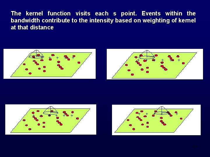
The kernel function visits each s point. Events within the bandwidth contribute to the intensity based on weighting of kernel at that distance 61

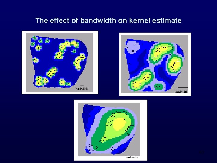
The effect of bandwidth on kernel estimate 1. For large , will appear flat and local features will be obscured. 2. If is small then tends to become a collection of spikes centered on the si. Changing the bandwidth allows you to look at the variation in intensity at different scales. For exploratory purposes it is useful to test various bandwidths to examine the change in intensity at different scales 62

The effect of bandwidth on kernel estimate 63

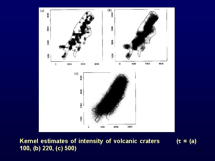
Kernel estimates of intensity of volcanic craters 100, (b) 220, (c) 500) ( = (a) 64

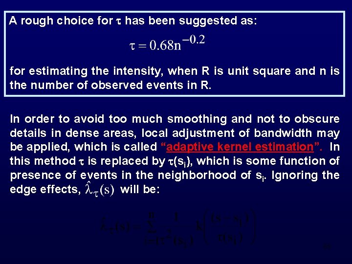
A rough choice for has been suggested as: for estimating the intensity, when R is unit square and n is the number of observed events in R. In order to avoid too much smoothing and not to obscure details in dense areas, local adjustment of bandwidth may be applied, which is called “adaptive kernel estimation”. In this method is replaced by (si), which is some function of presence of events in the neighborhood of si. Ignoring the edge effects, will be: 65

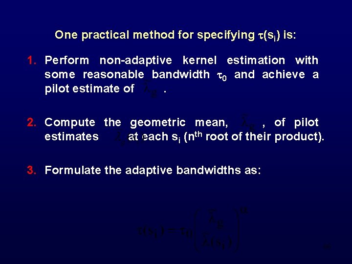
One practical method for specifying (si) is: 1. Perform non-adaptive kernel estimation with some reasonable bandwidth 0 and achieve a pilot estimate of. 2. Compute the geometric mean, , of pilot estimates at each si (nth root of their product). 3. Formulate the adaptive bandwidths as: 66

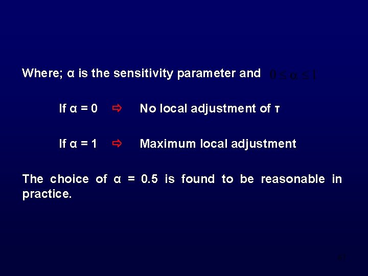
Where; α is the sensitivity parameter and If α = 0 No local adjustment of τ If α = 1 Maximum local adjustment The choice of α = 0. 5 is found to be reasonable in practice. 67

68

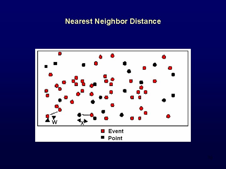
Nearest Neighbor Distance This method is designed for investigating the second order properties of the spatial point process and focuses on the relationship between inter-event distances. In this method the nearest neighbor event-event distance (W) and the nearest neighbor point-event distance (X) will constitute the basic area of interest. W: The distance between a randomly selected event in the study region a nearest neighboring event. X: The distance between a randomly selected point in the study region an the nearest neighboring event W X Mapped point pattern Sampled point pattern 69

Nearest Neighbor Distance 70

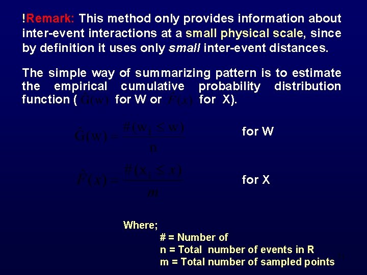
!Remark: This method only provides information about inter-event interactions at a small physical scale, since by definition it uses only small inter-event distances. The simple way of summarizing pattern is to estimate the empirical cumulative probability distribution function ( for W or for X). for W for X Where; # = Number of n = Total number of events in R 71 m = Total number of sampled points

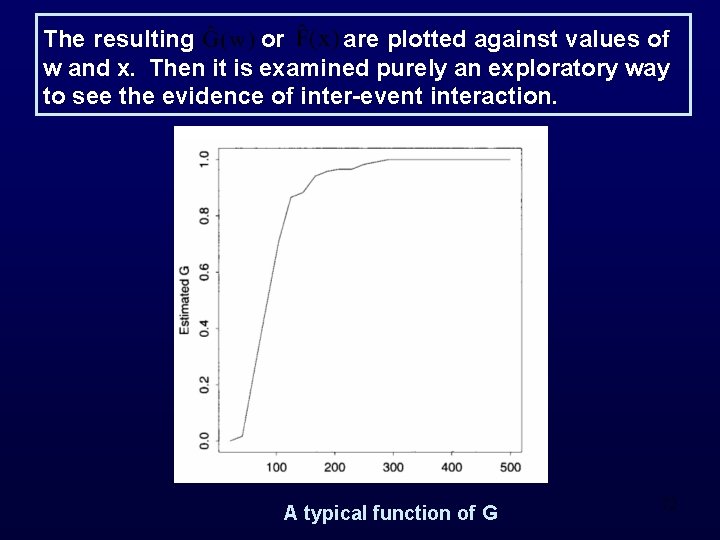
The resulting or are plotted against values of w and x. Then it is examined purely an exploratory way to see the evidence of inter-event interaction. A typical function of G 72

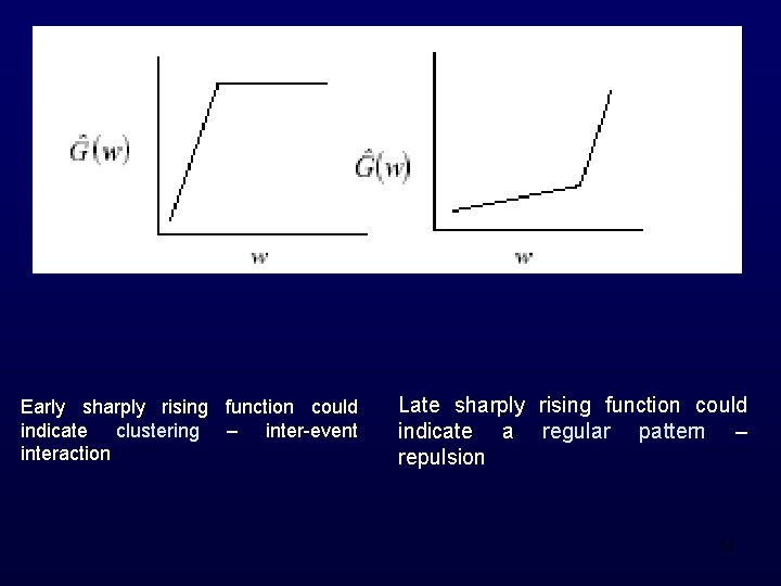
Interpretations for the plots of or v If the distribution function ( or ) climbs very steeply in the early part of its range before flattening out, then the indication would be an observed probability of short as opposed to long nearest neighbor distances, which suggest clustering. v If distribution function ( or ) climbs very steeply in the later part of its range, then the suggestion might be one of inter-event regularity. 73

Early sharply rising function could indicate clustering – inter-event interaction Late sharply rising function could indicate a regular pattern – repulsion 74

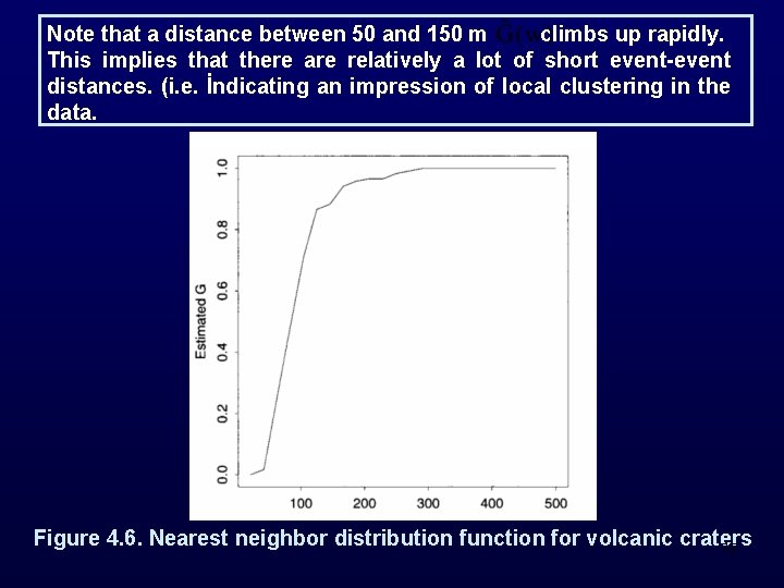
Note that a distance between 50 and 150 m climbs up rapidly. This implies that there are relatively a lot of short event-event distances. (i. e. İndicating an impression of local clustering in the data. Figure 4. 6. Nearest neighbor distribution function for volcanic craters 75

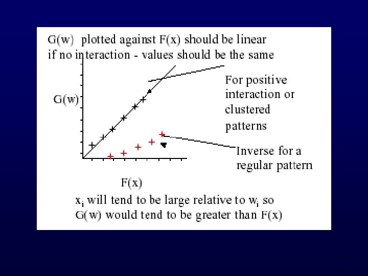
Another alternative would be to plot against . v. If there is no interaction these two distributions should be very similar and it is expected to obtain roughly a straight line in the plot. v. In the case of positive interaction or clustering, the point -event distances (xi) will tend to be large relative to event distances (wi). Hence will have higher values than. The reverse holds for regular pattern. 76

77

Corrections for Edge Effects For boundary cases, because the nearest event may be located outside R, distance to the nearest event is unknown. If the nearest neighbor is taken to be the closest event within the study area, expected nearest neighbor distances will be greater for events located near the boundary than for events located near the center of the study region Thus estimates based on nearest neighbor statistics will be biased without some edge correction applied 78

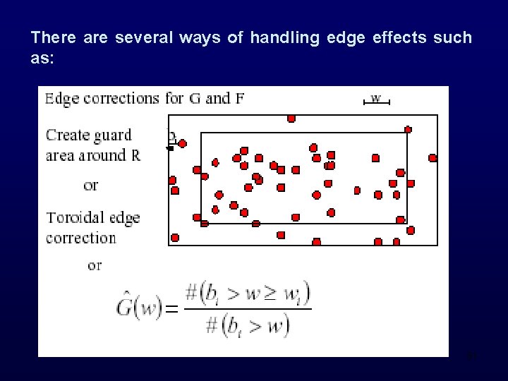
There are several ways of handling edge effects such as: 1. The problem can be overcome by constructing a guard area inside the perimeter of R. The nearest neighbor distances are not used for events within the guard area. But events in the guard area are allowed as neighbors of any event from the rest of R. 2. Another approach to the problem can be employed when the study region is rectangle, which is called use of toroidal edge correction. The study region is regarded as the central region of a 3× 3 grid of rectangle regions, each identical to the study region. i. e. top of the study region is assumed to be joined to the bottom and the left to the right. Events in the copies are allowed to be neighbors of any events (points) which are selected in the study region. 79

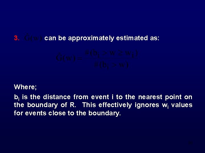
3. can be approximately estimated as: Where; bi is the distance from event i to the nearest point on the boundary of R. This effectively ignores wi values for events close to the boundary. 80

There are several ways of handling edge effects such as: 81

The K function The nearest neighbor distances method uses distances only closest events and therefore only considers the smallest scales of pattern. Information on larger scales of pattern is ignored. An alternative approach is to use an estimate of the reduced second moment measure or K function of the observed process, which provides a more effective summary of spatial dependence over a wider range of scales. 82

Properties of the K function 1. The K function represents information at various scales of pattern. 2. It involves use of precise location of events and includes all event-event distances, not just nearest neighbor distances. 3. The theoretical form of K(h) is not only used for various possible spatial point pattern models, but also suggest specific models to present it and to estimate the parameters of such models. 83

The K function FRemark: When examining spatial dependence over small scales in R, an implicit assumption is made, which is assuming that the process is isotropic over such scales. However, second order properties are not necessarily constant over the considered scale and may be confused with first order effects. E. g. If it is clear that there is large scale variation in intensity of given point pattern over the whole of R, this is truly a first order effect not a result of spatial dependence. In this case it is convinient to study second order effects over scales in R small enough for the assumption of isotropy to hold. If there is no variation in the intensity, it is appropriate to study the second order effects over larger scales in the study region. 84

The K function relates to the second order properties of an isotropic process. However, if it is used in a situation where there are large scale first order effects, then any spatial dependence it may indicate could be due to first order effects rather than to interaction effects. In such a case, it is better to examine smaller sub regions of R, since isotropy can reasonably be assumed to hold. 85

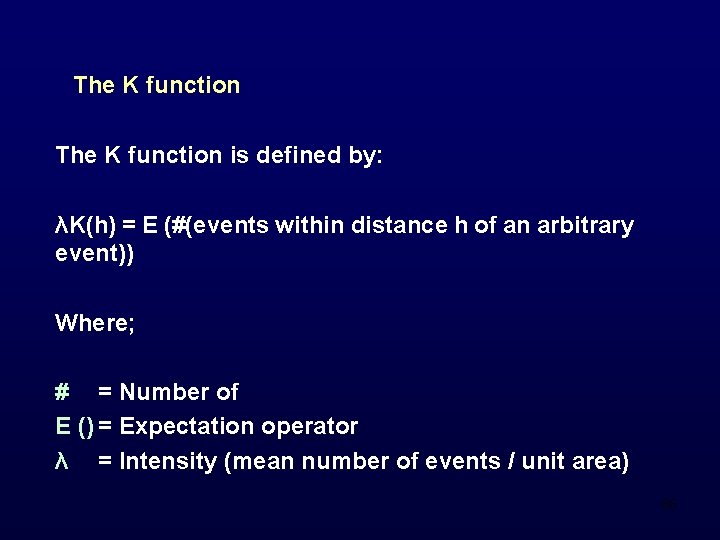
The K function is defined by: λK(h) = E (#(events within distance h of an arbitrary event)) Where; # = Number of E () = Expectation operator λ = Intensity (mean number of events / unit area) 86

The K function 87

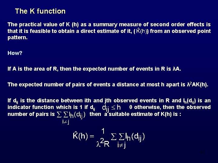
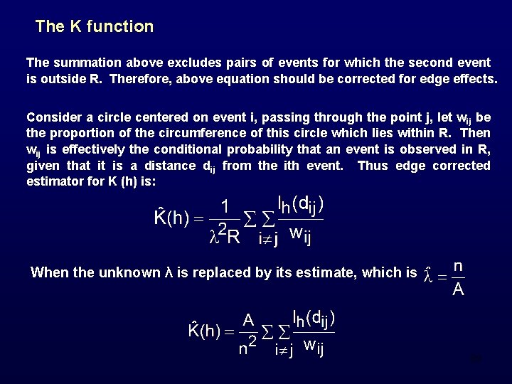
The K function The practical value of K (h) as a summary measure of second order effects is that it is feasible to obtain a direct estimate of it, ( ) from an observed point pattern. How? If A is the area of R, then the expected number of events in R is λA. The expected number of pairs of events a distance at most h apart is λ 2 AK(h). If dij is the distance between ith and jth observed events in R and Ih(dij) is an indicator function which is 1 if dij 0 otherwise, then the observed number of pairs is then a suitable estimate of K(h) is : 88

The K function The summation above excludes pairs of events for which the second event is outside R. Therefore, above equation should be corrected for edge effects. Consider a circle centered on event i, passing through the point j, let wij be the proportion of the circumference of this circle which lies within R. Then wij is effectively the conditional probability that an event is observed in R, given that it is a distance dij from the ith event. Thus edge corrected estimator for K (h) is: When the unknown λ is replaced by its estimate, which is 89

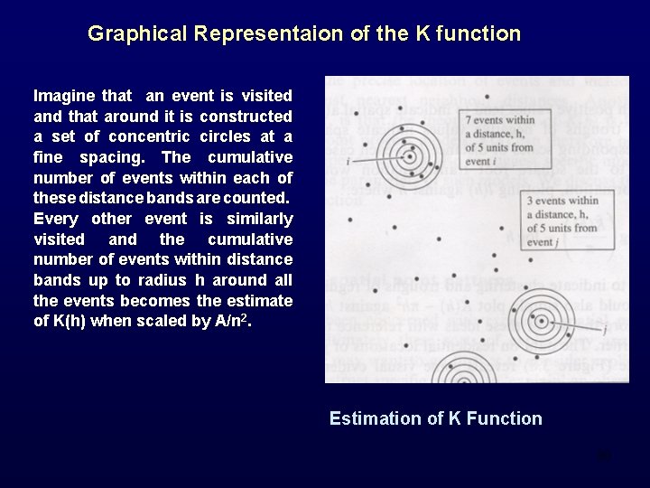
Graphical Representaion of the K function Imagine that an event is visited and that around it is constructed a set of concentric circles at a fine spacing. The cumulative number of events within each of these distance bands are counted. Every other event is similarly visited and the cumulative number of events within distance bands up to radius h around all the events becomes the estimate of K(h) when scaled by A/n 2. Estimation of K Function 90

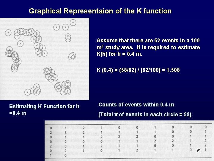
Graphical Representaion of the K function Assume that there are 62 events in a 100 m 2 study area. It is required to estimate K(h) for h = 0. 4 m. K (0. 4) = (58/62) / (62/100) = 1. 508 Estimating K Function for h =0. 4 m Counts of events within 0. 4 m (Total # of events in each circle = 58) 91

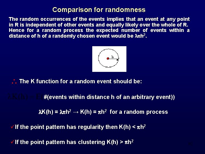
Comparison for randomness The random occurrences of the events implies that an event at any point in R is independent of other events and equally likely over the whole of R. Hence for a random process the expected number of events within a distance of h of a randomly chosen event would be h 2. The K function for a random event should be: #(events within distance h of an arbitrary event)) K(h) = h 2 → K(h) = h 2 for a random process üIf the point pattern has regularity then K(h) < h 2 üIf the point pattern has clustering K(h) > h 2 92

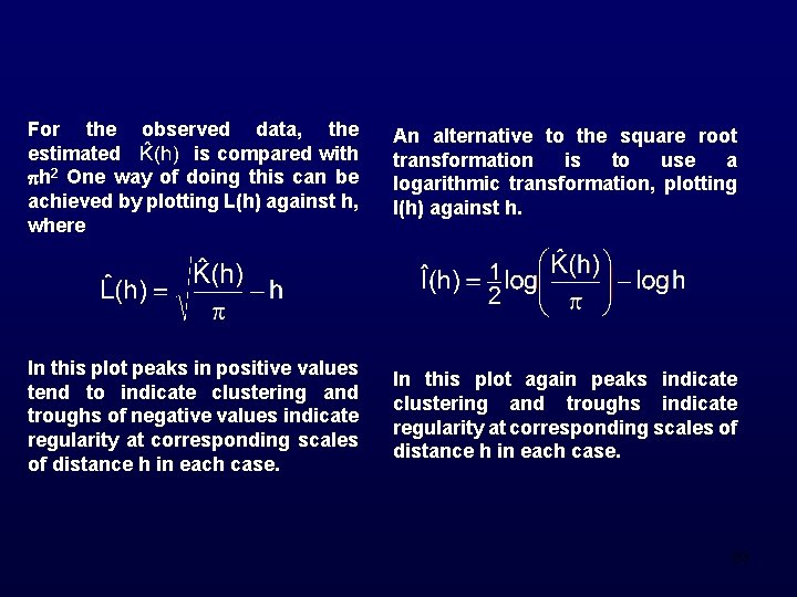
For the observed data, the estimated is compared with h 2 One way of doing this can be achieved by plotting L(h) against h, where An alternative to the square root transformation is to use a logarithmic transformation, plotting I(h) against h. In this plot peaks in positive values tend to indicate clustering and troughs of negative values indicate regularity at corresponding scales of distance h in each case. In this plot again peaks indicate clustering and troughs indicate regularity at corresponding scales of distance h in each case. 93

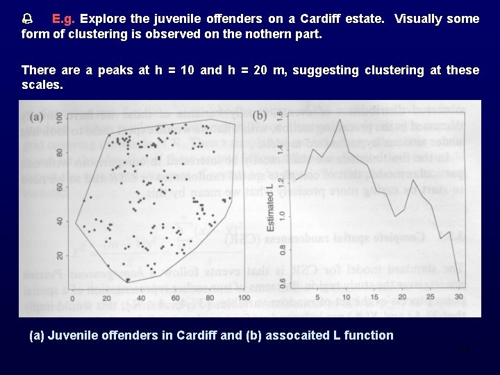
E. g. Explore the juvenile offenders on a Cardiff estate. Visually some form of clustering is observed on the nothern part. There a peaks at h = 10 and h = 20 m, suggesting clustering at these scales. (a) Juvenile offenders in Cardiff and (b) assocaited L function 94