Spatial and Temporal Data Mining Classification and Prediction

Spatial and Temporal Data Mining Classification and Prediction Vasileios Megalooikonomou (based on notes by Jiawei Han and Micheline Kamber)

Agenda • • • What is classification? What is prediction? Issues regarding classification and prediction Classification by decision tree induction Bayesian Classification by backpropagation Classification based on concepts from association rule mining Other Classification Methods Prediction Classification accuracy Summary

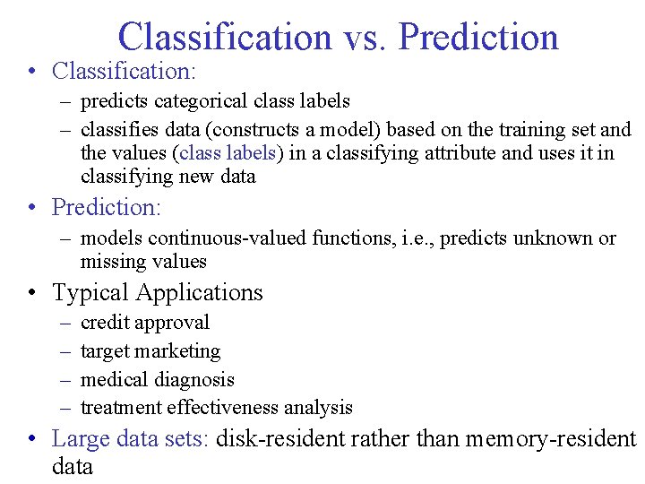
Classification vs. Prediction • Classification: – predicts categorical class labels – classifies data (constructs a model) based on the training set and the values (class labels) in a classifying attribute and uses it in classifying new data • Prediction: – models continuous-valued functions, i. e. , predicts unknown or missing values • Typical Applications – – credit approval target marketing medical diagnosis treatment effectiveness analysis • Large data sets: disk-resident rather than memory-resident data

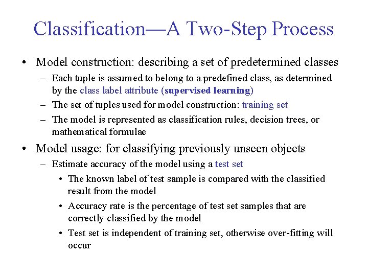
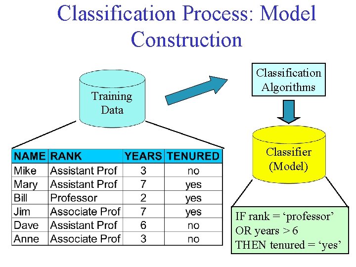
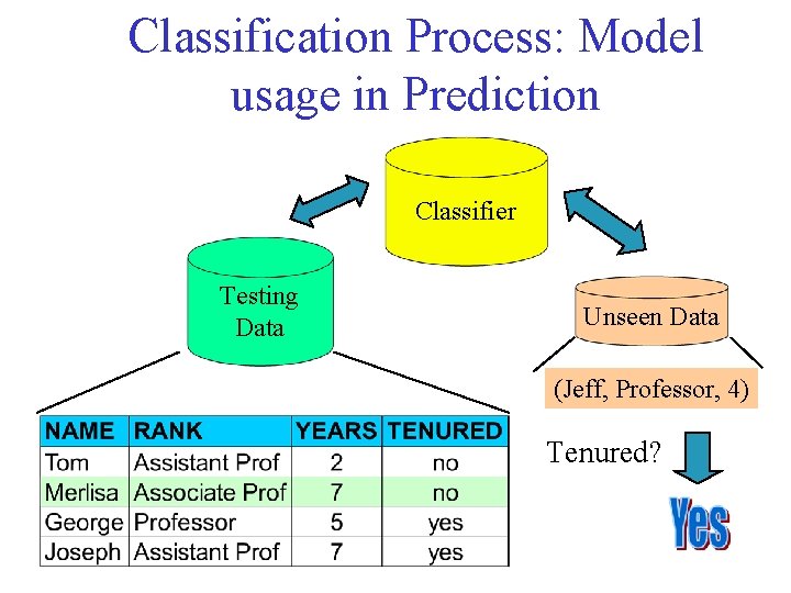
Classification—A Two-Step Process • Model construction: describing a set of predetermined classes – Each tuple is assumed to belong to a predefined class, as determined by the class label attribute (supervised learning) – The set of tuples used for model construction: training set – The model is represented as classification rules, decision trees, or mathematical formulae • Model usage: for classifying previously unseen objects – Estimate accuracy of the model using a test set • The known label of test sample is compared with the classified result from the model • Accuracy rate is the percentage of test set samples that are correctly classified by the model • Test set is independent of training set, otherwise over-fitting will occur

Classification Process: Model Construction Training Data Classification Algorithms Classifier (Model) IF rank = ‘professor’ OR years > 6 THEN tenured = ‘yes’

Classification Process: Model usage in Prediction Classifier Testing Data Unseen Data (Jeff, Professor, 4) Tenured?

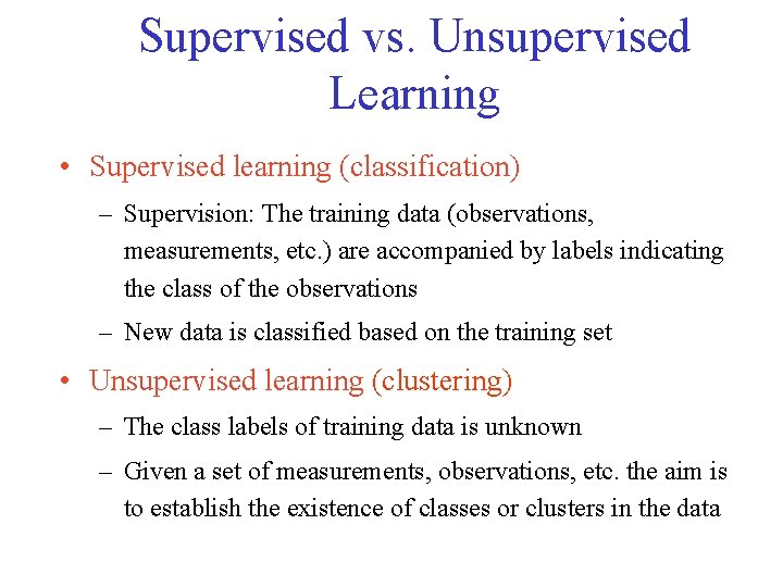
Supervised vs. Unsupervised Learning • Supervised learning (classification) – Supervision: The training data (observations, measurements, etc. ) are accompanied by labels indicating the class of the observations – New data is classified based on the training set • Unsupervised learning (clustering) – The class labels of training data is unknown – Given a set of measurements, observations, etc. the aim is to establish the existence of classes or clusters in the data

Agenda • • • What is classification? What is prediction? Issues regarding classification and prediction Classification by decision tree induction Bayesian Classification by backpropagation Classification based on concepts from association rule mining Other Classification Methods Prediction Classification accuracy Summary

Issues regarding classification and prediction: Data Preparation • Data cleaning – Preprocess data in order to reduce noise and handle missing values • Relevance analysis (feature selection) – Remove the irrelevant or redundant attributes • Data transformation – Generalize and/or normalize data

Issues regarding classification and prediction: Evaluating Classification Methods • Predictive accuracy • Speed and scalability – time to construct the model – time to use the model – efficiency in disk-resident databases • Robustness – handling noise and missing values • Interpretability: – understanding and insight provided by the model • Goodness of rules – decision tree size – compactness of classification rules

Agenda • • • What is classification? What is prediction? Issues regarding classification and prediction Classification by decision tree induction Bayesian Classification by backpropagation Classification based on concepts from association rule mining Other Classification Methods Prediction Classification accuracy Summary

Classification by Decision Tree Induction • Decision trees basics (covered earlier) • Attribute selection measure: – Information gain (ID 3/C 4. 5) • All attributes are assumed to be categorical • Can be modified for continuous-valued attributes – Gini index (IBM Intelligent. Miner) • All attributes are assumed continuous-valued • Assume there exist several possible split values for each attribute • May need other tools, such as clustering, to get the possible split values • Can be modified for categorical attributes • Avoid overfitting • Extract classification rules from trees

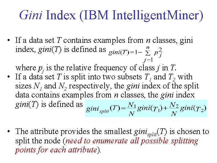
Gini Index (IBM Intelligent. Miner) • If a data set T contains examples from n classes, gini index, gini(T) is defined as where pj is the relative frequency of class j in T. • If a data set T is split into two subsets T 1 and T 2 with sizes N 1 and N 2 respectively, the gini index of the split data contains examples from n classes, the gini index gini(T) is defined as • The attribute provides the smallest ginisplit(T) is chosen to split the node (need to enumerate all possible splitting points for each attribute).

Approaches to Determine the Final Tree Size • Separate training (2/3) and testing (1/3) sets • Use cross validation, e. g. , 10 -fold cross validation • Use all the data for training – but apply a statistical test (e. g. , chi-square) to estimate whether expanding or pruning a node may improve the entire distribution • Use minimum description length (MDL) principle: – halting growth of the tree when the encoding is minimized

Enhancements to basic decision tree induction • Allow for continuous-valued attributes – Dynamically define new discrete-valued attributes that partition the continuous attribute value into a discrete set of intervals • Handle missing attribute values – Assign the most common value of the attribute – Assign probability to each of the possible values • Attribute construction – Create new attributes based on existing ones that are sparsely represented – This reduces fragmentation, repetition, and replication

Classification in Large Databases • Classification—a classical problem extensively studied by statisticians and machine learning researchers • Scalability: Classifying data sets with millions of examples and hundreds of attributes with reasonable speed • Why decision tree induction in data mining? – relatively faster learning speed (than other classification methods) – convertible to simple and easy to understand classification rules – can use SQL queries for accessing databases – comparable classification accuracy with other methods

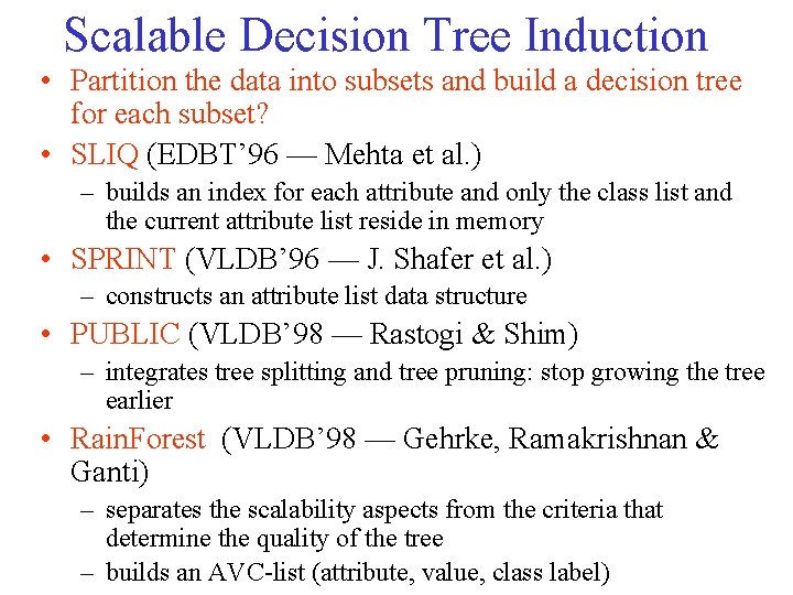
Scalable Decision Tree Induction • Partition the data into subsets and build a decision tree for each subset? • SLIQ (EDBT’ 96 — Mehta et al. ) – builds an index for each attribute and only the class list and the current attribute list reside in memory • SPRINT (VLDB’ 96 — J. Shafer et al. ) – constructs an attribute list data structure • PUBLIC (VLDB’ 98 — Rastogi & Shim) – integrates tree splitting and tree pruning: stop growing the tree earlier • Rain. Forest (VLDB’ 98 — Gehrke, Ramakrishnan & Ganti) – separates the scalability aspects from the criteria that determine the quality of the tree – builds an AVC-list (attribute, value, class label)

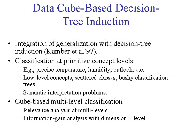
Data Cube-Based Decision. Tree Induction • Integration of generalization with decision-tree induction (Kamber et al’ 97). • Classification at primitive concept levels – E. g. , precise temperature, humidity, outlook, etc. – Low-level concepts, scattered classes, bushy classificationtrees – Semantic interpretation problems. • Cube-based multi-level classification – Relevance analysis at multi-levels. – Information-gain analysis with dimension + level.

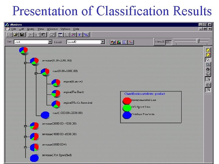
Presentation of Classification Results

Agenda • • • What is classification? What is prediction? Issues regarding classification and prediction Classification by decision tree induction Bayesian Classification by backpropagation Classification based on concepts from association rule mining Other Classification Methods Prediction Classification accuracy Summary

Bayesian Classification: Why? • Probabilistic learning: – Calculate explicit probabilities for hypothesis – Among the most practical approaches to certain types of learning problems • Incremental: – Each training example can incrementally increase/decrease the probability that a hypothesis is correct. – Prior knowledge can be combined with observed data. • Probabilistic prediction: – Predict multiple hypotheses, weighted by their probabilities • Standard: – Even when Bayesian methods are computationally intractable, they can provide a standard of optimal decision making against which other methods can be measured

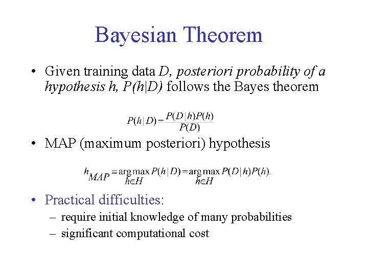
Bayesian Theorem • Given training data D, posteriori probability of a hypothesis h, P(h|D) follows the Bayes theorem • MAP (maximum posteriori) hypothesis • Practical difficulties: – require initial knowledge of many probabilities – significant computational cost

Bayesian classification • The classification problem may be formalized using a-posteriori probabilities: • P(C|X) = prob. that the sample tuple X=<x 1, …, xk> is of class C. • E. g. P(class=N | outlook=sunny, windy=true, …) • Idea: assign to sample X the class label C such that P(C|X) is maximal

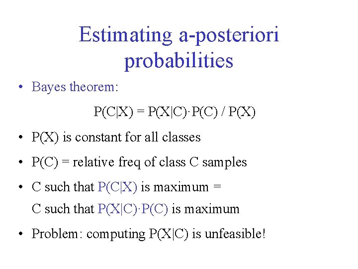
Estimating a-posteriori probabilities • Bayes theorem: P(C|X) = P(X|C)·P(C) / P(X) • P(X) is constant for all classes • P(C) = relative freq of class C samples • C such that P(C|X) is maximum = C such that P(X|C)·P(C) is maximum • Problem: computing P(X|C) is unfeasible!

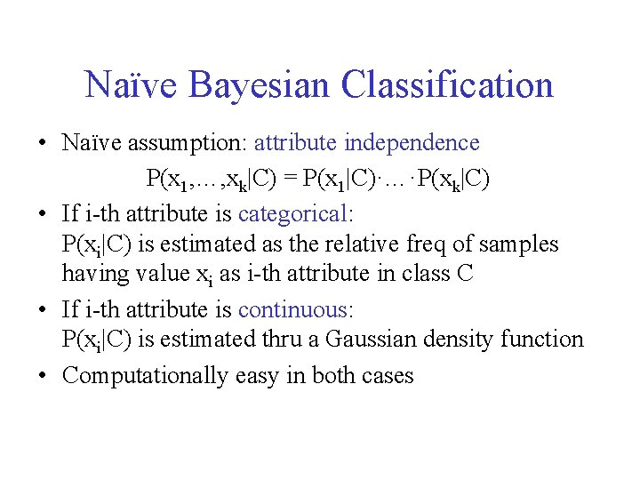
Naïve Bayesian Classification • Naïve assumption: attribute independence P(x 1, …, xk|C) = P(x 1|C)·…·P(xk|C) • If i-th attribute is categorical: P(xi|C) is estimated as the relative freq of samples having value xi as i-th attribute in class C • If i-th attribute is continuous: P(xi|C) is estimated thru a Gaussian density function • Computationally easy in both cases

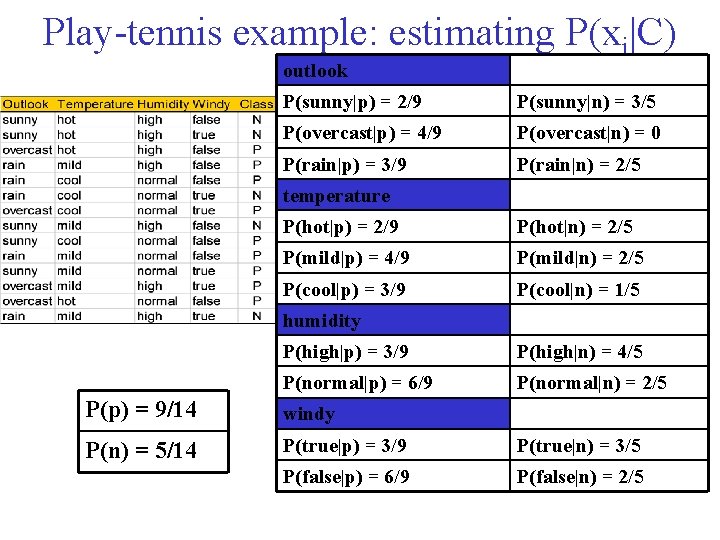
Play-tennis example: estimating P(xi|C) outlook P(sunny|p) = 2/9 P(sunny|n) = 3/5 P(overcast|p) = 4/9 P(overcast|n) = 0 P(rain|p) = 3/9 P(rain|n) = 2/5 temperature P(hot|p) = 2/9 P(hot|n) = 2/5 P(mild|p) = 4/9 P(mild|n) = 2/5 P(cool|p) = 3/9 P(cool|n) = 1/5 humidity P(high|p) = 3/9 P(high|n) = 4/5 P(normal|p) = 6/9 P(normal|n) = 2/5 P(p) = 9/14 windy P(n) = 5/14 P(true|p) = 3/9 P(true|n) = 3/5 P(false|p) = 6/9 P(false|n) = 2/5

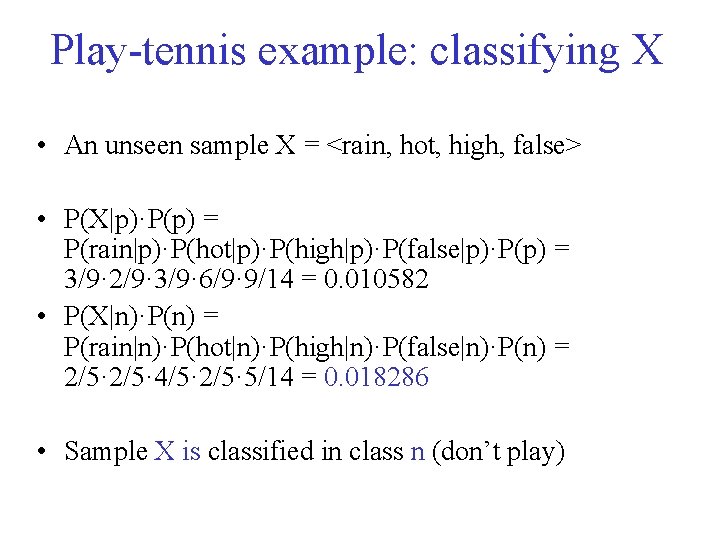
Play-tennis example: classifying X • An unseen sample X = <rain, hot, high, false> • P(X|p)·P(p) = P(rain|p)·P(hot|p)·P(high|p)·P(false|p)·P(p) = 3/9· 2/9· 3/9· 6/9· 9/14 = 0. 010582 • P(X|n)·P(n) = P(rain|n)·P(hot|n)·P(high|n)·P(false|n)·P(n) = 2/5· 4/5· 2/5· 5/14 = 0. 018286 • Sample X is classified in class n (don’t play)

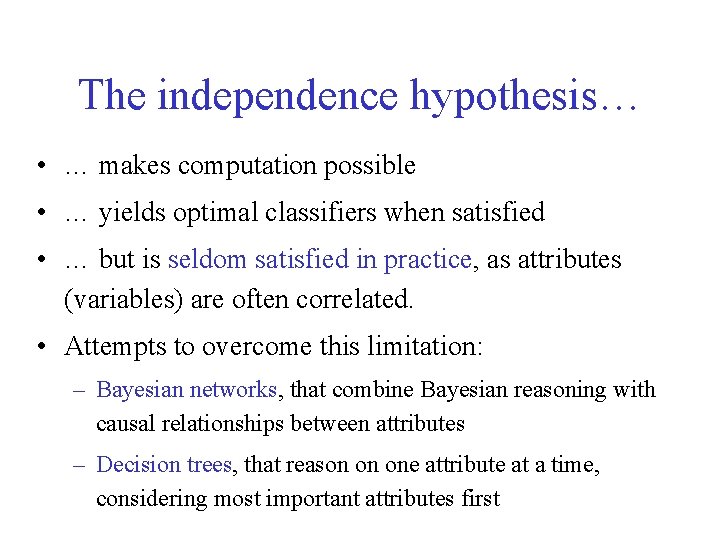
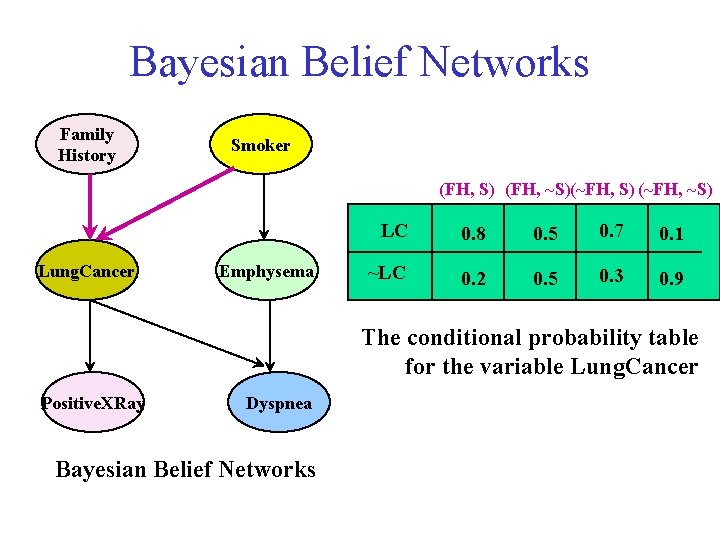
The independence hypothesis… • … makes computation possible • … yields optimal classifiers when satisfied • … but is seldom satisfied in practice, as attributes (variables) are often correlated. • Attempts to overcome this limitation: – Bayesian networks, that combine Bayesian reasoning with causal relationships between attributes – Decision trees, that reason on one attribute at a time, considering most important attributes first

Bayesian Belief Networks Family History Smoker (FH, S) (FH, ~S)(~FH, S) (~FH, ~S) Lung. Cancer Emphysema LC 0. 8 0. 5 0. 7 0. 1 ~LC 0. 2 0. 5 0. 3 0. 9 The conditional probability table for the variable Lung. Cancer Positive. XRay Dyspnea Bayesian Belief Networks

Bayesian Belief Networks • Bayesian belief network allows a subset of the variables conditionally independent • A graphical model of causal relationships • Several cases of learning Bayesian belief networks – Given both network structure and all the variables: easy – Given network structure but only some variables – When the network structure is not known in advance • Classification process returns a prob. distribution for the class label attribute (not just a single class label)

Agenda • • • What is classification? What is prediction? Issues regarding classification and prediction Classification by decision tree induction Bayesian Classification by backpropagation Classification based on concepts from association rule mining Other Classification Methods Prediction Classification accuracy Summary

Neural Networks A set of connected input/output units where each connection has a weight associated with it • Advantages – prediction accuracy is generally high – robust, works when training examples contain errors – output may be discrete, real-valued, or a vector of several discrete or real-valued attributes – fast evaluation of the learned target function • Criticism – long training time – require (typically empirically determined) parameters (e. g. network topology) – difficult to understand the learned function (weights) – not easy to incorporate domain knowledge

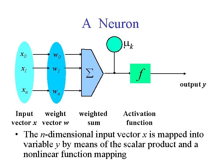
x 0 w 0 x 1 w 1 xn A Neuron - mk å f wn Input weight vector x vector w weighted sum output y Activation function • The n-dimensional input vector x is mapped into variable y by means of the scalar product and a nonlinear function mapping

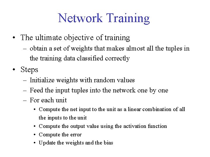
Network Training • The ultimate objective of training – obtain a set of weights that makes almost all the tuples in the training data classified correctly • Steps – Initialize weights with random values – Feed the input tuples into the network one by one – For each unit • Compute the net input to the unit as a linear combination of all the inputs to the unit • Compute the output value using the activation function • Compute the error • Update the weights and the bias

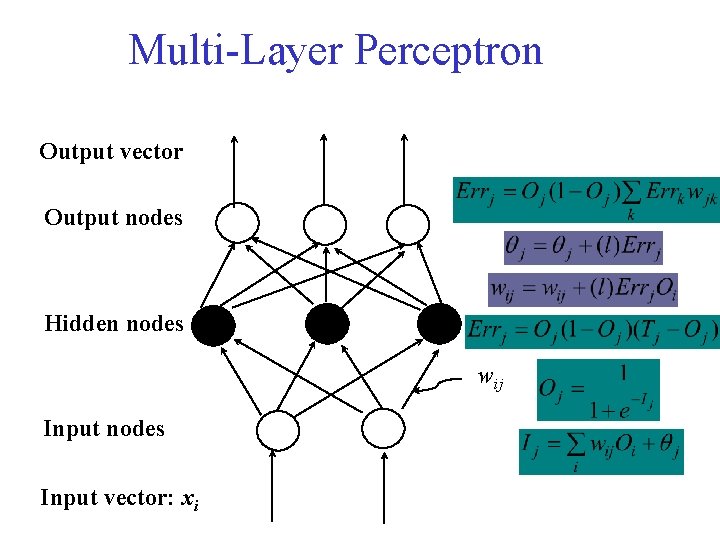
Multi-Layer Perceptron Output vector Output nodes Hidden nodes wij Input nodes Input vector: xi

Agenda • • • What is classification? What is prediction? Issues regarding classification and prediction Classification by decision tree induction Bayesian Classification by backpropagation Support Vector Machines Classification based on concepts from association rule mining Other Classification Methods Prediction Classification accuracy Summary

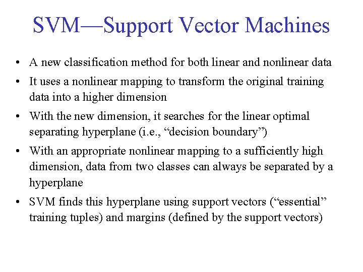
SVM—Support Vector Machines • A new classification method for both linear and nonlinear data • It uses a nonlinear mapping to transform the original training data into a higher dimension • With the new dimension, it searches for the linear optimal separating hyperplane (i. e. , “decision boundary”) • With an appropriate nonlinear mapping to a sufficiently high dimension, data from two classes can always be separated by a hyperplane • SVM finds this hyperplane using support vectors (“essential” training tuples) and margins (defined by the support vectors)

SVM—History and Applications • Vapnik and colleagues (1992)—groundwork from Vapnik & Chervonenkis’ statistical learning theory in 1960 s • Features: training can be slow but accuracy is high owing to their ability to model complex nonlinear decision boundaries (margin maximization) • Used both for classification and prediction • Applications: – handwritten digit recognition, object recognition, speaker identification, benchmarking time-series prediction tests

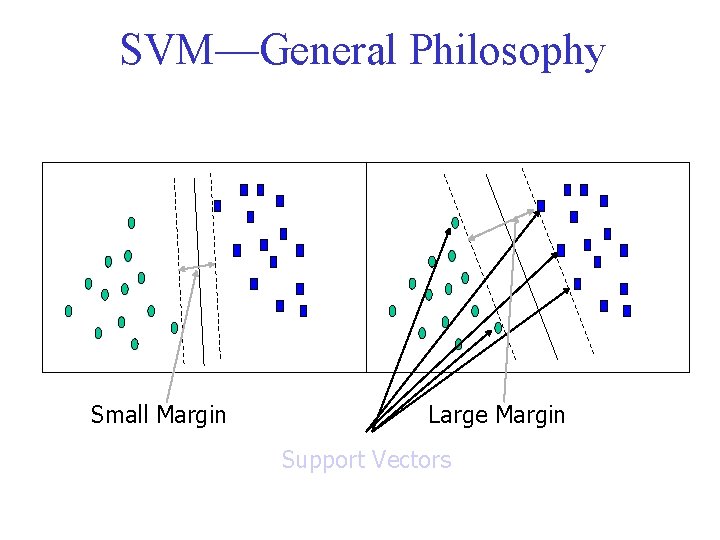
SVM—General Philosophy Small Margin Large Margin Support Vectors

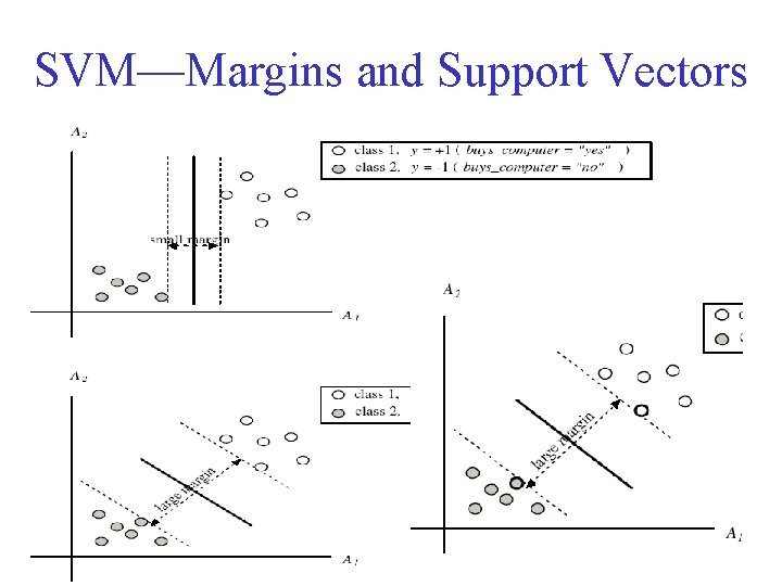
SVM—Margins and Support Vectors

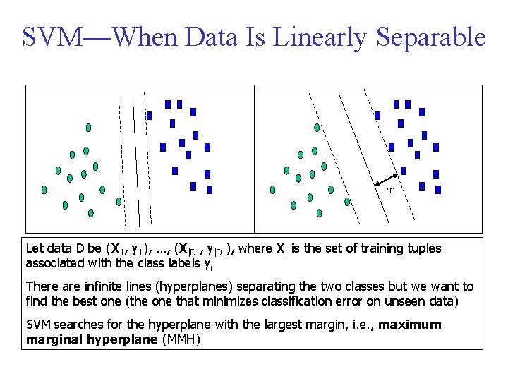
SVM—When Data Is Linearly Separable m Let data D be (X 1, y 1), …, (X|D|, y|D|), where Xi is the set of training tuples associated with the class labels yi There are infinite lines (hyperplanes) separating the two classes but we want to find the best one (the one that minimizes classification error on unseen data) SVM searches for the hyperplane with the largest margin, i. e. , maximum marginal hyperplane (MMH)

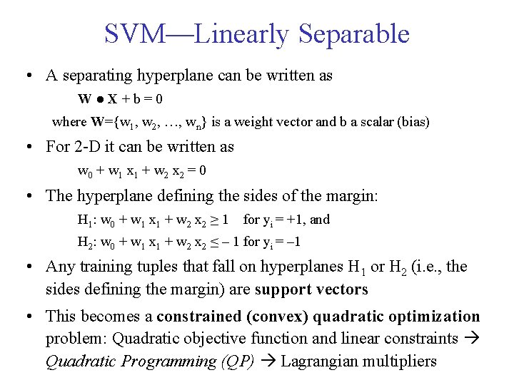
SVM—Linearly Separable • A separating hyperplane can be written as W ● X + b = 0 where W={w 1, w 2, …, wn} is a weight vector and b a scalar (bias) • For 2 -D it can be written as w 0 + w 1 x 1 + w 2 x 2 = 0 • The hyperplane defining the sides of the margin: H 1: w 0 + w 1 x 1 + w 2 x 2 ≥ 1 for yi = +1, and H 2: w 0 + w 1 x 1 + w 2 x 2 ≤ – 1 for yi = – 1 • Any training tuples that fall on hyperplanes H 1 or H 2 (i. e. , the sides defining the margin) are support vectors • This becomes a constrained (convex) quadratic optimization problem: Quadratic objective function and linear constraints Quadratic Programming (QP) Lagrangian multipliers

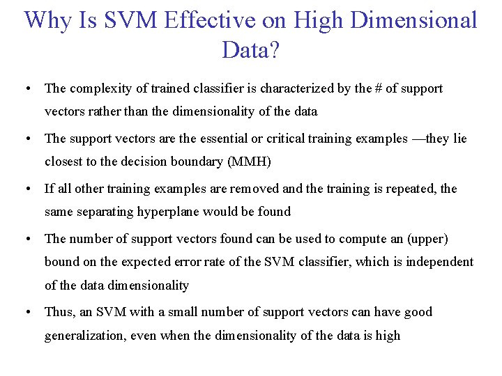
Why Is SVM Effective on High Dimensional Data? • The complexity of trained classifier is characterized by the # of support vectors rather than the dimensionality of the data • The support vectors are the essential or critical training examples —they lie closest to the decision boundary (MMH) • If all other training examples are removed and the training is repeated, the same separating hyperplane would be found • The number of support vectors found can be used to compute an (upper) bound on the expected error rate of the SVM classifier, which is independent of the data dimensionality • Thus, an SVM with a small number of support vectors can have good generalization, even when the dimensionality of the data is high

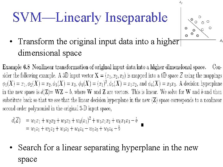
SVM—Linearly Inseparable • Transform the original input data into a higher dimensional space • Search for a linear separating hyperplane in the new space

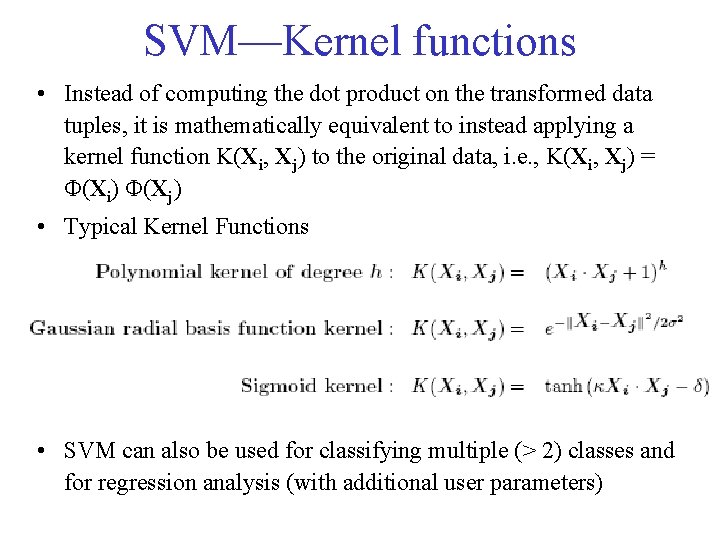
SVM—Kernel functions • Instead of computing the dot product on the transformed data tuples, it is mathematically equivalent to instead applying a kernel function K(Xi, Xj) to the original data, i. e. , K(Xi, Xj) = Φ(Xi) Φ(Xj) • Typical Kernel Functions • SVM can also be used for classifying multiple (> 2) classes and for regression analysis (with additional user parameters)

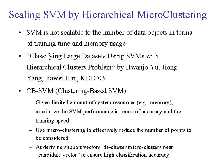
Scaling SVM by Hierarchical Micro. Clustering • SVM is not scalable to the number of data objects in terms of training time and memory usage • “Classifying Large Datasets Using SVMs with Hierarchical Clusters Problem” by Hwanjo Yu, Jiong Yang, Jiawei Han, KDD’ 03 • CB-SVM (Clustering-Based SVM) – Given limited amount of system resources (e. g. , memory), maximize the SVM performance in terms of accuracy and the training speed – Use micro-clustering to effectively reduce the number of points to be considered – At deriving support vectors, de-cluster micro-clusters near “candidate vector” to ensure high classification accuracy

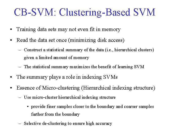
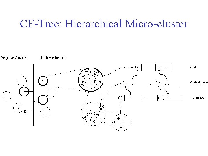
CB-SVM: Clustering-Based SVM • Training data sets may not even fit in memory • Read the data set once (minimizing disk access) – Construct a statistical summary of the data (i. e. , hierarchical clusters) given a limited amount of memory – The statistical summary maximizes the benefit of learning SVM • The summary plays a role in indexing SVMs • Essence of Micro-clustering (Hierarchical indexing structure) – Use micro-cluster hierarchical indexing structure • provide finer samples closer to the boundary and coarser samples farther from the boundary – Selective de-clustering to ensure high accuracy

CF-Tree: Hierarchical Micro-cluster

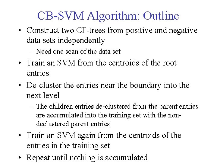
CB-SVM Algorithm: Outline • Construct two CF-trees from positive and negative data sets independently – Need one scan of the data set • Train an SVM from the centroids of the root entries • De-cluster the entries near the boundary into the next level – The children entries de-clustered from the parent entries are accumulated into the training set with the nondeclustered parent entries • Train an SVM again from the centroids of the entries in the training set • Repeat until nothing is accumulated

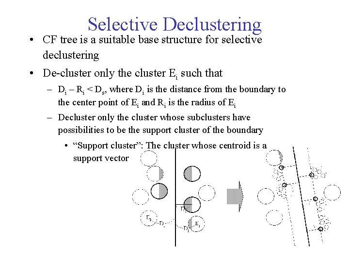
Selective Declustering • CF tree is a suitable base structure for selective declustering • De-cluster only the cluster Ei such that – Di – Ri < Ds, where Di is the distance from the boundary to the center point of Ei and Ri is the radius of Ei – Decluster only the cluster whose subclusters have possibilities to be the support cluster of the boundary • “Support cluster”: The cluster whose centroid is a support vector

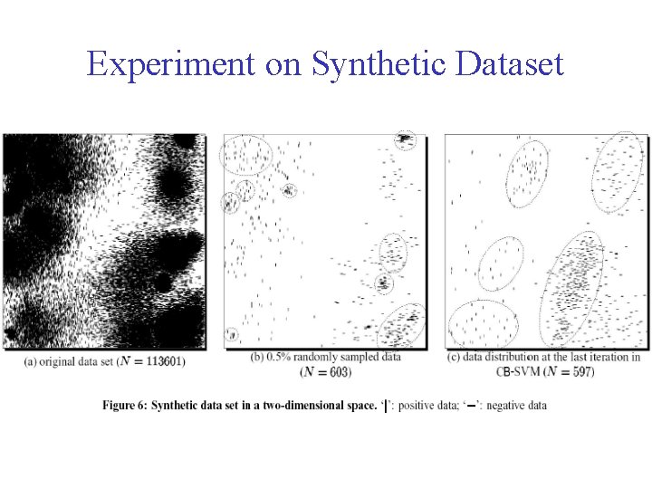
Experiment on Synthetic Dataset

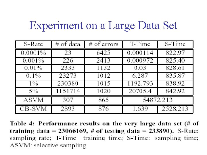
Experiment on a Large Data Set

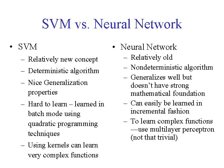
SVM vs. Neural Network • SVM – Relatively new concept – Deterministic algorithm – Nice Generalization properties – Hard to learn – learned in batch mode using quadratic programming techniques – Using kernels can learn very complex functions • Neural Network – Relatively old – Nondeterministic algorithm – Generalizes well but doesn’t have strong mathematical foundation – Can easily be learned in incremental fashion – To learn complex functions —use multilayer perceptron (not that trivial)

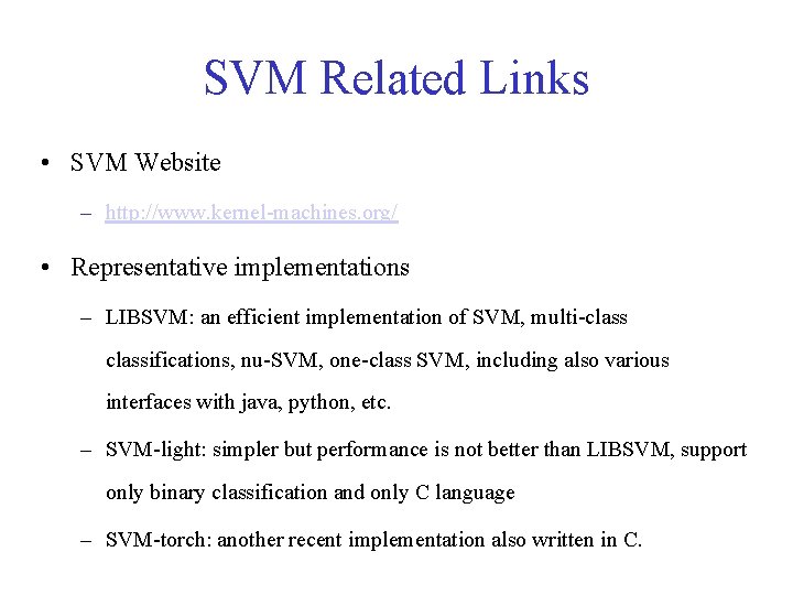
SVM Related Links • SVM Website – http: //www. kernel-machines. org/ • Representative implementations – LIBSVM: an efficient implementation of SVM, multi-classifications, nu-SVM, one-class SVM, including also various interfaces with java, python, etc. – SVM-light: simpler but performance is not better than LIBSVM, support only binary classification and only C language – SVM-torch: another recent implementation also written in C.

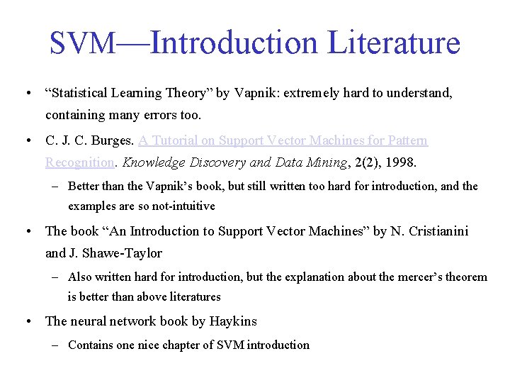
SVM—Introduction Literature • “Statistical Learning Theory” by Vapnik: extremely hard to understand, containing many errors too. • C. J. C. Burges. A Tutorial on Support Vector Machines for Pattern Recognition. Knowledge Discovery and Data Mining, 2(2), 1998. – Better than the Vapnik’s book, but still written too hard for introduction, and the examples are so not-intuitive • The book “An Introduction to Support Vector Machines” by N. Cristianini and J. Shawe-Taylor – Also written hard for introduction, but the explanation about the mercer’s theorem is better than above literatures • The neural network book by Haykins – Contains one nice chapter of SVM introduction

Agenda • • • What is classification? What is prediction? Issues regarding classification and prediction Classification by decision tree induction Bayesian Classification by backpropagation Support Vector Machines Classification based on concepts from association rule mining Other Classification Methods Prediction Classification accuracy Summary

Association-Based Classification • Several methods for association-based classification – ARCS: Quantitative association mining and clustering of association rules (Lent et al’ 97) • It beats C 4. 5 in (mainly) scalability and also accuracy – Associative classification: (Liu et al’ 98) • It mines high support and high confidence rules in the form of “cond_set => y”, where y is a class label – CAEP (Classification by aggregating emerging patterns) (Dong et al’ 99) • Emerging patterns (EPs): the itemsets whose support increases significantly from one class to another • Mine Eps based on minimum support and growth rate

Agenda • • • What is classification? What is prediction? Issues regarding classification and prediction Classification by decision tree induction Bayesian Classification by backpropagation Classification based on concepts from association rule mining Other Classification Methods Prediction Classification accuracy Summary

Other Classification Methods • k-nearest neighbor classifier • case-based reasoning • Genetic algorithm • Rough set approach • Fuzzy set approaches

Instance-Based Methods • Instance-based learning (or learning by ANALOGY): – Store training examples and delay the processing (“lazy evaluation”) until a new instance must be classified • Typical approaches – k-nearest neighbor approach • Instances represented as points in a Euclidean space. – Locally weighted regression • Constructs local approximation – Case-based reasoning • Uses symbolic representations and knowledge-based inference

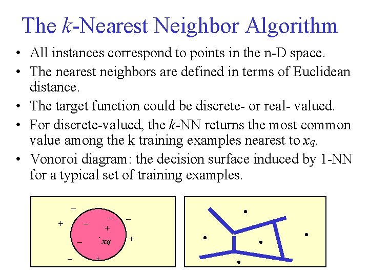
The k-Nearest Neighbor Algorithm • All instances correspond to points in the n-D space. • The nearest neighbors are defined in terms of Euclidean distance. • The target function could be discrete- or real- valued. • For discrete-valued, the k-NN returns the most common value among the k training examples nearest to xq. • Vonoroi diagram: the decision surface induced by 1 -NN for a typical set of training examples. _ _ + _ _ _ + . xq + . _ + . .

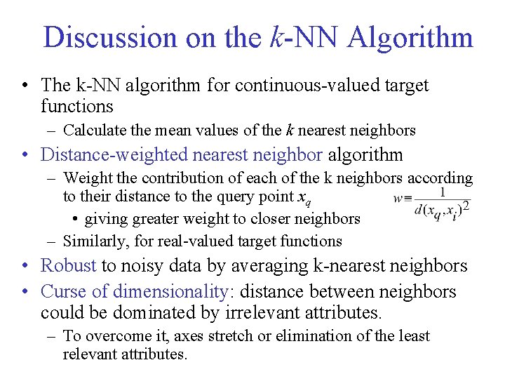
Discussion on the k-NN Algorithm • The k-NN algorithm for continuous-valued target functions – Calculate the mean values of the k nearest neighbors • Distance-weighted nearest neighbor algorithm – Weight the contribution of each of the k neighbors according to their distance to the query point xq • giving greater weight to closer neighbors – Similarly, for real-valued target functions • Robust to noisy data by averaging k-nearest neighbors • Curse of dimensionality: distance between neighbors could be dominated by irrelevant attributes. – To overcome it, axes stretch or elimination of the least relevant attributes.

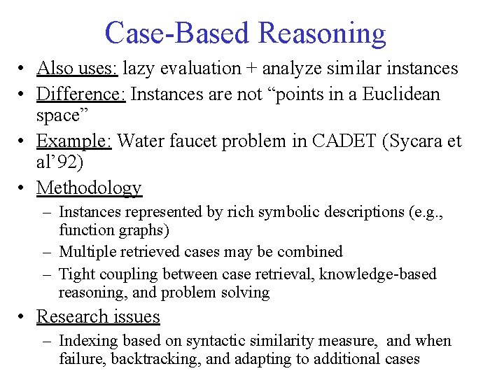
Case-Based Reasoning • Also uses: lazy evaluation + analyze similar instances • Difference: Instances are not “points in a Euclidean space” • Example: Water faucet problem in CADET (Sycara et al’ 92) • Methodology – Instances represented by rich symbolic descriptions (e. g. , function graphs) – Multiple retrieved cases may be combined – Tight coupling between case retrieval, knowledge-based reasoning, and problem solving • Research issues – Indexing based on syntactic similarity measure, and when failure, backtracking, and adapting to additional cases

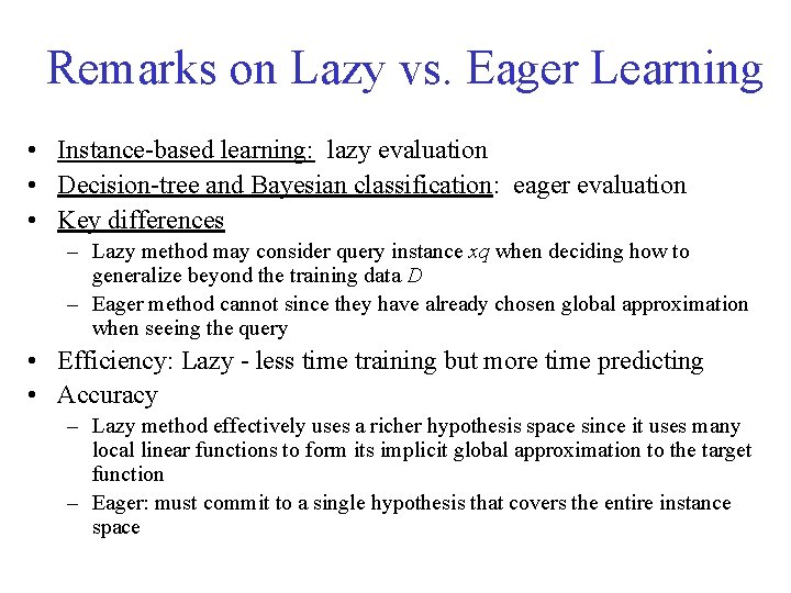
Remarks on Lazy vs. Eager Learning • Instance-based learning: lazy evaluation • Decision-tree and Bayesian classification: eager evaluation • Key differences – Lazy method may consider query instance xq when deciding how to generalize beyond the training data D – Eager method cannot since they have already chosen global approximation when seeing the query • Efficiency: Lazy - less time training but more time predicting • Accuracy – Lazy method effectively uses a richer hypothesis space since it uses many local linear functions to form its implicit global approximation to the target function – Eager: must commit to a single hypothesis that covers the entire instance space

Genetic Algorithms – Evolutionary Approach • GA: based on an analogy to biological evolution • Each rule is represented by a string of bits • An initial population is created consisting of randomly generated rules – e. g. , IF A 1 and Not A 2 then C 2 can be encoded as 100 • Based on the notion of survival of the fittest, a new population is formed to consists of the fittest rules and their offsprings • The fitness of a rule is represented by its classification accuracy on a set of training examples • Offsprings are generated by crossover and mutation

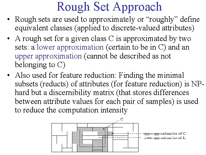
Rough Set Approach • Rough sets are used to approximately or “roughly” define equivalent classes (applied to discrete-valued attributes) • A rough set for a given class C is approximated by two sets: a lower approximation (certain to be in C) and an upper approximation (cannot be described as not belonging to C) • Also used for feature reduction: Finding the minimal subsets (reducts) of attributes (for feature reduction) is NPhard but a discernibility matrix (that stores differences between attribute values for each pair of samples) is used to reduce the computation intensity

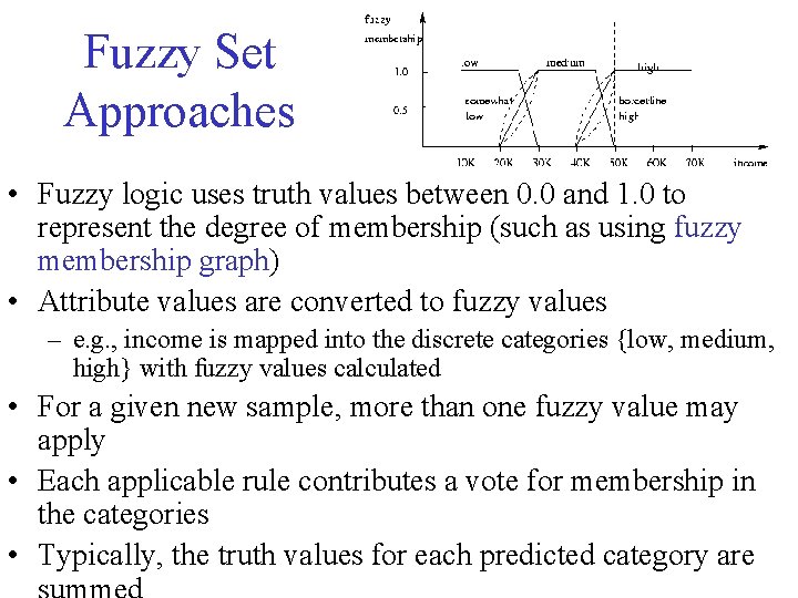
Fuzzy Set Approaches • Fuzzy logic uses truth values between 0. 0 and 1. 0 to represent the degree of membership (such as using fuzzy membership graph) • Attribute values are converted to fuzzy values – e. g. , income is mapped into the discrete categories {low, medium, high} with fuzzy values calculated • For a given new sample, more than one fuzzy value may apply • Each applicable rule contributes a vote for membership in the categories • Typically, the truth values for each predicted category are

Agenda • • • What is classification? What is prediction? Issues regarding classification and prediction Classification by decision tree induction Bayesian Classification by backpropagation Classification based on concepts from association rule mining Other Classification Methods Prediction Classification accuracy Summary

What Is Prediction? • Prediction is similar to classification – First, construct a model – Second, use model to predict unknown value • Major method for prediction is regression – Linear and multiple regression – Non-linear regression • Prediction is different from classification – Classification refers to predict categorical class label – Prediction models continuous-valued functions

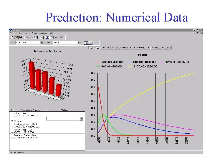
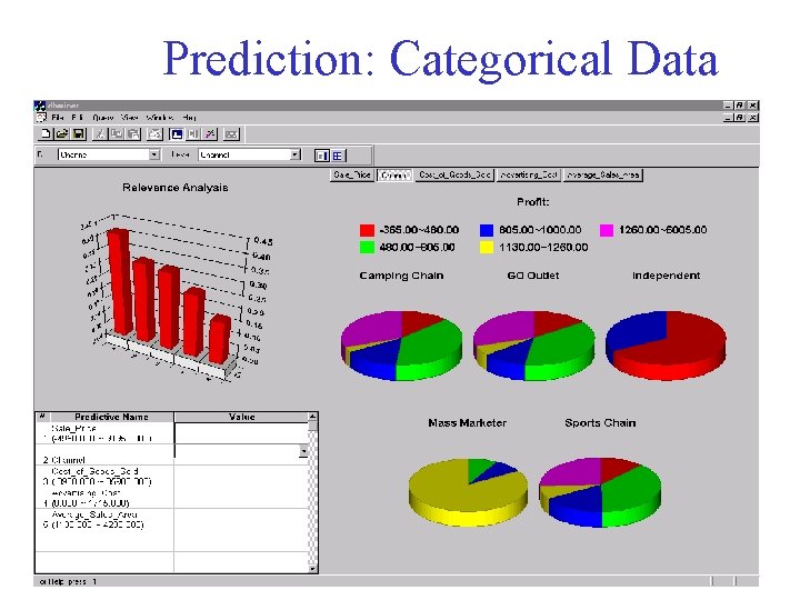
Predictive Modeling in Databases • Predictive modeling: – Predict data values or construct generalized linear models based on the database data. – predict value ranges or category distributions • Method outline: – – Minimal generalization Attribute relevance analysis Generalized linear model construction Prediction • Determine the major factors which influence the prediction – Data relevance analysis: uncertainty measurement, entropy analysis, expert judgement, etc. • Multi-level prediction: drill-down and roll-up analysis

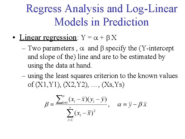
Regress Analysis and Log-Linear Models in Prediction • Linear regression: Y = + X – Two parameters , and specify the (Y-intercept and slope of the) line and are to be estimated by using the data at hand. – using the least squares criterion to the known values of (X 1, Y 1), (X 2, Y 2), …, (Xs, Ys)

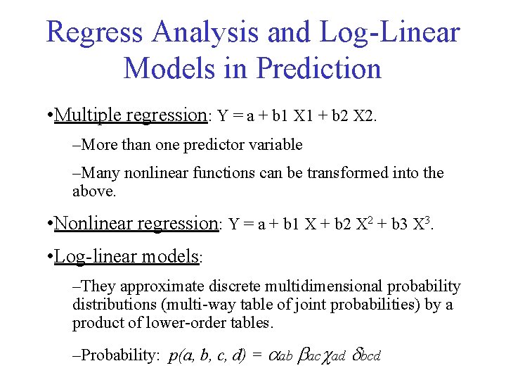
Regress Analysis and Log-Linear Models in Prediction • Multiple regression: Y = a + b 1 X 1 + b 2 X 2. –More than one predictor variable –Many nonlinear functions can be transformed into the above. • Nonlinear regression: Y = a + b 1 X + b 2 X 2 + b 3 X 3. • Log-linear models: –They approximate discrete multidimensional probability distributions (multi-way table of joint probabilities) by a product of lower-order tables. –Probability: p(a, b, c, d) = ab ac ad bcd

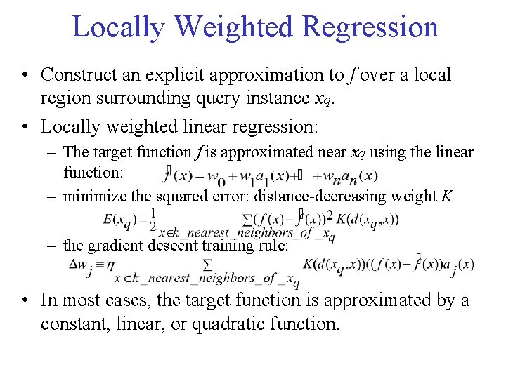
Locally Weighted Regression • Construct an explicit approximation to f over a local region surrounding query instance xq. • Locally weighted linear regression: – The target function f is approximated near xq using the linear function: – minimize the squared error: distance-decreasing weight K – the gradient descent training rule: • In most cases, the target function is approximated by a constant, linear, or quadratic function.

Prediction: Numerical Data

Prediction: Categorical Data

Agenda • • • What is classification? What is prediction? Issues regarding classification and prediction Classification by decision tree induction Bayesian Classification by backpropagation Classification based on concepts from association rule mining Other Classification Methods Prediction Classification accuracy Summary

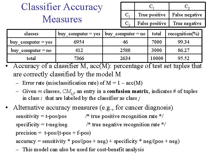
Classifier Accuracy Measures classes C 1 C 2 C 1 True positive False negative C 2 False positive True negative buy_computer = yes buy_computer = no total recognition(%) buy_computer = yes 6954 46 7000 99. 34 buy_computer = no 412 2588 3000 86. 27 total 7366 2634 10000 95. 52 • Accuracy of a classifier M, acc(M): percentage of test set tuples that are correctly classified by the model M – Error rate (misclassification rate) of M = 1 – acc(M) – Given m classes, CMi, j, an entry in a confusion matrix, indicates # of tuples in class i that are labeled by the classifier as class j • Alternative accuracy measures (e. g. , for cancer diagnosis) sensitivity = t-pos/pos /* true positive recognition rate */ specificity = t-neg/neg /* true negative recognition rate */ precision = t-pos/(t-pos + f-pos) accuracy = sensitivity * pos/(pos + neg) + specificity * neg/(pos + neg) – This model can also be used for cost-benefit analysis

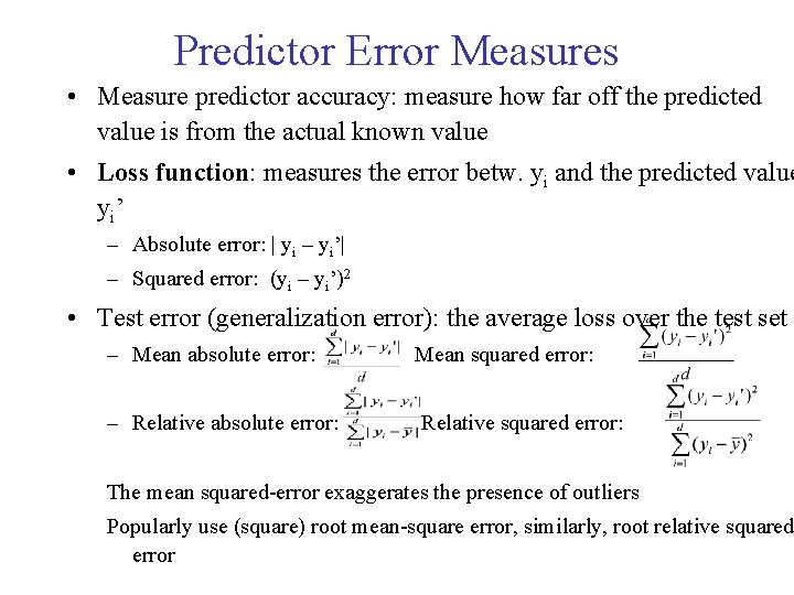
Predictor Error Measures • Measure predictor accuracy: measure how far off the predicted value is from the actual known value • Loss function: measures the error betw. yi and the predicted value yi’ – Absolute error: | yi – yi’| – Squared error: (yi – yi’)2 • Test error (generalization error): the average loss over the test set – Mean absolute error: Mean squared error: – Relative absolute error: Relative squared error: The mean squared-error exaggerates the presence of outliers Popularly use (square) root mean-square error, similarly, root relative squared error

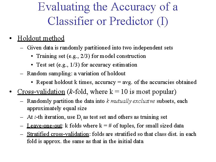
Evaluating the Accuracy of a Classifier or Predictor (I) • Holdout method – Given data is randomly partitioned into two independent sets • Training set (e. g. , 2/3) for model construction • Test set (e. g. , 1/3) for accuracy estimation – Random sampling: a variation of holdout • Repeat holdout k times, accuracy = avg. of the accuracies obtained • Cross-validation (k-fold, where k = 10 is most popular) – Randomly partition the data into k mutually exclusive subsets, each approximately equal size – At i-th iteration, use Di as test set and others as training set – Leave-one-out: k folds where k = # of tuples, for small sized data – Stratified cross-validation: folds are stratified so that class dist. in each fold is approx. the same as that in the initial data

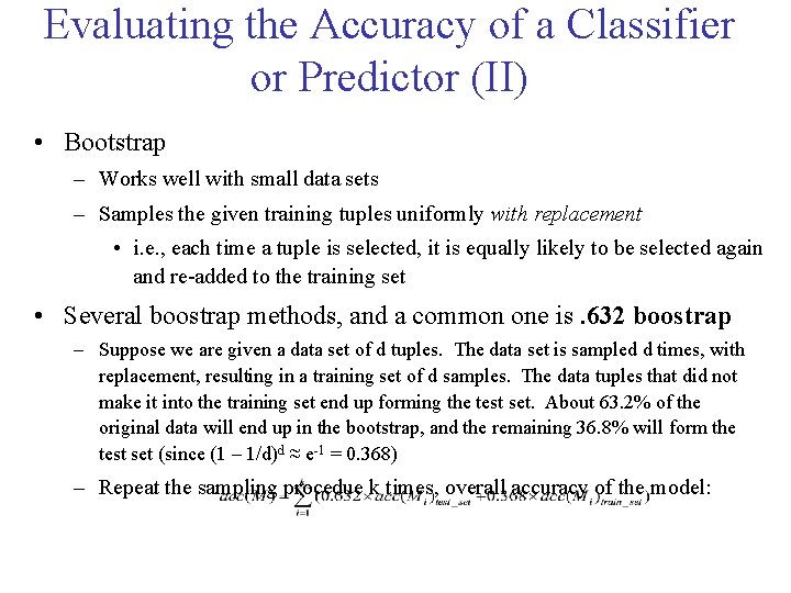
Evaluating the Accuracy of a Classifier or Predictor (II) • Bootstrap – Works well with small data sets – Samples the given training tuples uniformly with replacement • i. e. , each time a tuple is selected, it is equally likely to be selected again and re-added to the training set • Several boostrap methods, and a common one is. 632 boostrap – Suppose we are given a data set of d tuples. The data set is sampled d times, with replacement, resulting in a training set of d samples. The data tuples that did not make it into the training set end up forming the test set. About 63. 2% of the original data will end up in the bootstrap, and the remaining 36. 8% will form the test set (since (1 – 1/d)d ≈ e-1 = 0. 368) – Repeat the sampling procedue k times, overall accuracy of the model:

Agenda • • • What is classification? What is prediction? Issues regarding classification and prediction Classification by decision tree induction Bayesian Classification by backpropagation Classification based on concepts from association rule mining Other Classification Methods Prediction Classification accuracy Ensemble methods, Bagging, Boosting Summary

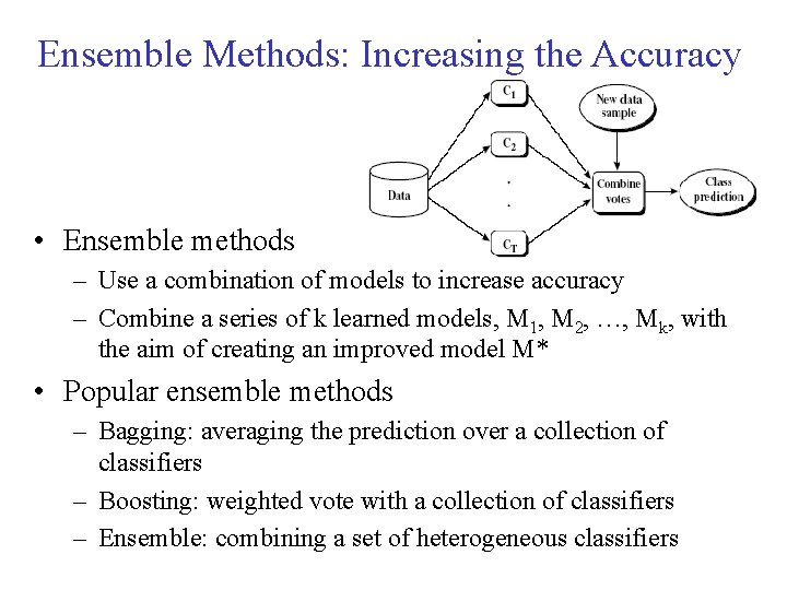
Ensemble Methods: Increasing the Accuracy • Ensemble methods – Use a combination of models to increase accuracy – Combine a series of k learned models, M 1, M 2, …, Mk, with the aim of creating an improved model M* • Popular ensemble methods – Bagging: averaging the prediction over a collection of classifiers – Boosting: weighted vote with a collection of classifiers – Ensemble: combining a set of heterogeneous classifiers

Bagging: Boostrap Aggregation • Analogy: Diagnosis based on multiple doctors’ majority vote • Training – Given a set D of d tuples, at each iteration i, a training set Di of d tuples is sampled with replacement from D (i. e. , boostrap) – A classifier model Mi is learned for each training set Di • Classification: classify an unknown sample X – Each classifier Mi returns its class prediction – The bagged classifier M* counts the votes and assigns the class with the most votes to X • Prediction: can be applied to the prediction of continuous values by taking the average value of each prediction for a given test tuple • Accuracy – Often significant better than a single classifier derived from D – For noise data: not considerably worse, more robust – Proved improved accuracy in prediction

Boosting • Analogy: Consult several doctors, based on a combination of weighted diagnoses—weight assigned based on the previous diagnosis accuracy • How boosting works? – Weights are assigned to each training tuple – A series of k classifiers is iteratively learned – After a classifier Mi is learned, the weights are updated to allow the subsequent classifier, Mi+1, to pay more attention to the training tuples that were misclassified by Mi – The final M* combines the votes of each individual classifier, where the weight of each classifier's vote is a function of its accuracy • The boosting algorithm can be extended for the prediction of continuous values • Comparing with bagging: boosting tends to achieve greater accuracy, but it also risks overfitting the model to misclassified data

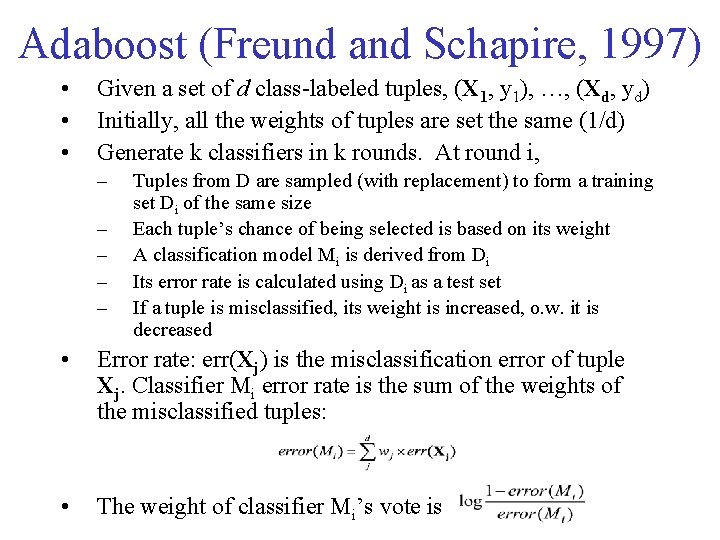
Adaboost (Freund and Schapire, 1997) • • • Given a set of d class-labeled tuples, (X 1, y 1), …, (Xd, yd) Initially, all the weights of tuples are set the same (1/d) Generate k classifiers in k rounds. At round i, – – – Tuples from D are sampled (with replacement) to form a training set Di of the same size Each tuple’s chance of being selected is based on its weight A classification model Mi is derived from Di Its error rate is calculated using Di as a test set If a tuple is misclassified, its weight is increased, o. w. it is decreased • Error rate: err(Xj) is the misclassification error of tuple Xj. Classifier Mi error rate is the sum of the weights of the misclassified tuples: • The weight of classifier Mi’s vote is

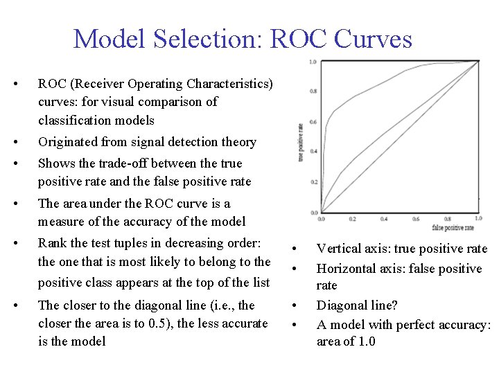
Model Selection: ROC Curves • ROC (Receiver Operating Characteristics) curves: for visual comparison of classification models • Originated from signal detection theory • Shows the trade-off between the true positive rate and the false positive rate • The area under the ROC curve is a measure of the accuracy of the model • Rank the test tuples in decreasing order: the one that is most likely to belong to the positive class appears at the top of the list • The closer to the diagonal line (i. e. , the closer the area is to 0. 5), the less accurate is the model • • Vertical axis: true positive rate Horizontal axis: false positive rate Diagonal line? A model with perfect accuracy: area of 1. 0

Agenda • • • What is classification? What is prediction? Issues regarding classification and prediction Classification by decision tree induction Bayesian Classification by backpropagation Classification based on concepts from association rule mining Other Classification Methods Prediction Classification accuracy Summary

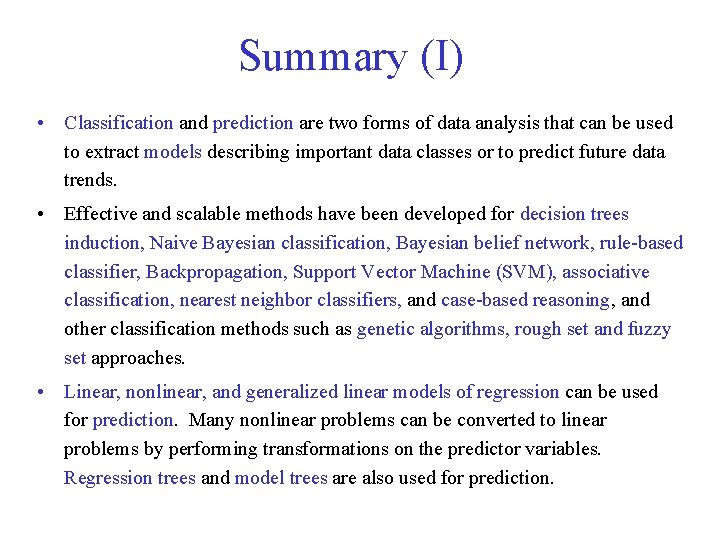
Summary (I) • Classification and prediction are two forms of data analysis that can be used to extract models describing important data classes or to predict future data trends. • Effective and scalable methods have been developed for decision trees induction, Naive Bayesian classification, Bayesian belief network, rule-based classifier, Backpropagation, Support Vector Machine (SVM), associative classification, nearest neighbor classifiers, and case-based reasoning, and other classification methods such as genetic algorithms, rough set and fuzzy set approaches. • Linear, nonlinear, and generalized linear models of regression can be used for prediction. Many nonlinear problems can be converted to linear problems by performing transformations on the predictor variables. Regression trees and model trees are also used for prediction.

Summary (II) • Stratified k-fold cross-validation is a recommended method for accuracy estimation. Bagging and boosting can be used to increase overall accuracy by learning and combining a series of individual models. • Significance tests and ROC curves are useful for model selection • There have been numerous comparisons of the different classification and prediction methods, and the matter remains a research topic • No single method has been found to be superior over all others for all data sets • Issues such as accuracy, training time, robustness, interpretability, and scalability must be considered and can involve trade-offs, further complicating the quest for an overall superior method

References (1) • • C. Apte and S. Weiss. Data mining with decision trees and decision rules. Future Generation Computer Systems, 13, 1997. • • P. K. Chan and S. J. Stolfo. Learning arbiter and combiner trees from partitioned data for scaling machine learning. KDD'95. • • • J. Gehrke, R. Ramakrishnan, and V. Ganti. Rainforest: A framework for fast decision tree construction of large datasets. VLDB’ 98. • D. Heckerman, D. Geiger, and D. M. Chickering. Learning Bayesian networks: The combination of knowledge and statistical data. Machine Learning, 1995. • M. Kamber, L. Winstone, W. Gong, S. Cheng, and J. Han. Generalization and decision tree induction: Efficient classification in data mining. RIDE'97. • • B. Liu, W. Hsu, and Y. Ma. Integrating Classification and Association Rule. KDD'98. C. M. Bishop, Neural Networks for Pattern Recognition. Oxford University Press, 1995. L. Breiman, J. Friedman, R. Olshen, and C. Stone. Classification and Regression Trees. Wadsworth International Group, 1984. C. J. C. Burges. A Tutorial on Support Vector Machines for Pattern Recognition. Data Mining and Knowledge Discovery, 2(2): 121 -168, 1998. W. Cohen. Fast effective rule induction. ICML'95. G. Cong, K. -L. Tan, A. K. H. Tung, and X. Xu. Mining top-k covering rule groups for gene expression data. SIGMOD'05. A. J. Dobson. An Introduction to Generalized Linear Models. Chapman and Hall, 1990. G. Dong and J. Li. Efficient mining of emerging patterns: Discovering trends and differences. KDD'99. R. O. Duda, P. E. Hart, and D. G. Stork. Pattern Classification, 2 ed. John Wiley and Sons, 2001 U. M. Fayyad. Branching on attribute values in decision tree generation. AAAI’ 94. Y. Freund and R. E. Schapire. A decision-theoretic generalization of on-line learning and an application to boosting. J. Computer and System Sciences, 1997. J. Gehrke, V. Gant, R. Ramakrishnan, and W. -Y. Loh, BOAT -- Optimistic Decision Tree Construction. SIGMOD'99. T. Hastie, R. Tibshirani, and J. Friedman. The Elements of Statistical Learning: Data Mining, Inference, and Prediction. Springer-Verlag, 2001. W. Li, J. Han, and J. Pei, CMAR: Accurate and Efficient Classification Based on Multiple Class-Association Rules, ICDM'01.

References (2) • T. -S. Lim, W. -Y. Loh, and Y. -S. Shih. A comparison of prediction accuracy, complexity, and training time of thirty-three old and new classification algorithms. Machine Learning, 2000. • J. Magidson. The Chaid approach to segmentation modeling: Chi-squared automatic interaction detection. In R. P. Bagozzi, editor, Advanced Methods of Marketing Research, Blackwell Business, 1994. • M. Mehta, R. Agrawal, and J. Rissanen. SLIQ : A fast scalable classifier for data mining. EDBT'96. • T. M. Mitchell. Machine Learning. Mc. Graw Hill, 1997. • S. K. Murthy, Automatic Construction of Decision Trees from Data: A Multi-Disciplinary Survey, Data Mining and Knowledge Discovery 2(4): 345 -389, 1998 • J. R. Quinlan. Induction of decision trees. Machine Learning, 1: 81 -106, 1986. • J. R. Quinlan and R. M. Cameron-Jones. FOIL: A midterm report. ECML’ 93. • J. R. Quinlan. C 4. 5: Programs for Machine Learning. Morgan Kaufmann, 1993. • J. R. Quinlan. Bagging, boosting, and c 4. 5. AAAI'96. • • • R. Rastogi and K. Shim. Public: A decision tree classifier that integrates building and pruning. VLDB’ 98. • • S. M. Weiss and N. Indurkhya. Predictive Data Mining. Morgan Kaufmann, 1997. J. Shafer, R. Agrawal, and M. Mehta. SPRINT : A scalable parallel classifier for data mining. VLDB’ 96. J. W. Shavlik and T. G. Dietterich. Readings in Machine Learning. Morgan Kaufmann, 1990. P. Tan, M. Steinbach, and V. Kumar. Introduction to Data Mining. Addison Wesley, 2005. S. M. Weiss and C. A. Kulikowski. Computer Systems that Learn: Classification and Prediction Methods from Statistics, Neural Nets, Machine Learning, and Expert Systems. Morgan Kaufman, 1991. I. H. Witten and E. Frank. Data Mining: Practical Machine Learning Tools and Techniques, 2 ed. Morgan Kaufmann, 2005. X. Yin and J. Han. CPAR: Classification based on predictive association rules. SDM'03 H. Yu, J. Yang, and J. Han. Classifying large data sets using SVM with hierarchical clusters. KDD'03.