Sorting HKOI Training Team Advanced 2006 01 21

Sorting HKOI Training Team (Advanced) 2006 -01 -21

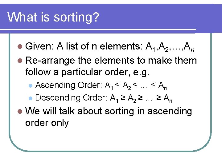
What is sorting? l Given: A list of n elements: A 1, A 2, …, An l Re-arrange the elements to make them follow a particular order, e. g. Ascending Order: A 1 ≤ A 2 ≤ … ≤ An l Descending Order: A 1 ≥ A 2 ≥ … ≥ An l l We will talk about sorting in ascending order only

Why is sorting needed? l Some algorithms works only when data is sorted l e. g. binary search l Better l presentation of data Often required by problem setters, to reduce workload in judging

Why learn Sorting Algorithms? l C++ STL already provided a sort() function l Unfortunately, no such implementation for Pascal l This is a minor point, though

Why learn Sorting Algorithms? l Most importantly, OI problems does not directly ask for sorting, but its solution may be closely linked with sorting algorithms l In most cases, C++ STL sort() is useless. You still need to write your own “sort” l So… it is important to understand the idea behind each algorithm, and also their strengths and weaknesses

Some Sorting Algorithms… l l l l l Bubble Sort Insertion Sort Selection Sort Shell Sort Heap Sort Merge Sort Quick Sort Counting Sort Radix Sort How many of them do you know?

Bubble, Insertion, Selection… l Simple, in terms of Idea, and l Implementation l l Unfortunately, l they are inefficient O(n 2) – not good if N is large l Algorithms being taught today are far more efficient than these

Shell Sort l Named after its inventor, Donald Shell l Observation: Insertion Sort is very efficient when n is small l when the list is almost sorted l

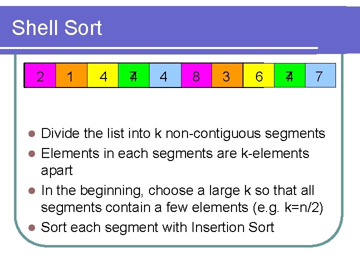
Shell Sort 2 1 4 7 4 4 8 3 6 4 7 7 Divide the list into k non-contiguous segments l Elements in each segments are k-elements apart l In the beginning, choose a large k so that all segments contain a few elements (e. g. k=n/2) l Sort each segment with Insertion Sort l

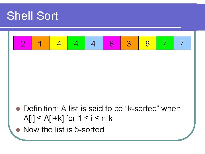
Shell Sort 2 1 4 4 4 8 3 6 7 7 Definition: A list is said to be “k-sorted” when A[i] ≤ A[i+k] for 1 ≤ i ≤ n-k l Now the list is 5 -sorted l

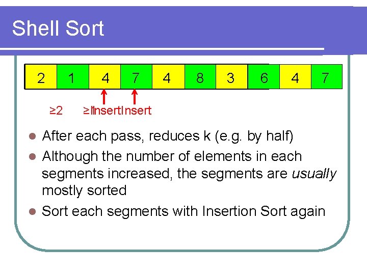
Shell Sort 2 1 ≥ 2 4 7 4 8 3 6 4 7 ≥ 1 Insert After each pass, reduces k (e. g. by half) l Although the number of elements in each segments increased, the segments are usually mostly sorted l Sort each segments with Insertion Sort again l

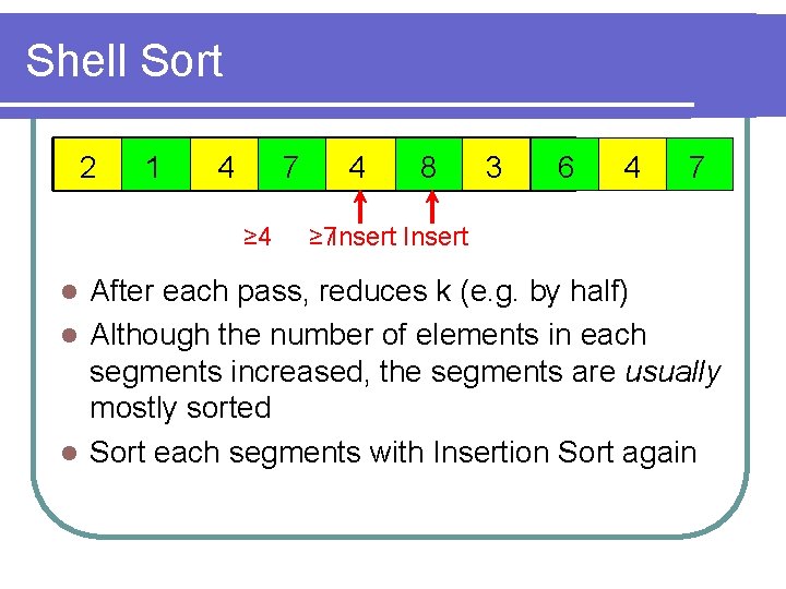
Shell Sort 2 1 4 7 ≥ 4 4 8 3 6 4 7 ≥ 7 Insert After each pass, reduces k (e. g. by half) l Although the number of elements in each segments increased, the segments are usually mostly sorted l Sort each segments with Insertion Sort again l

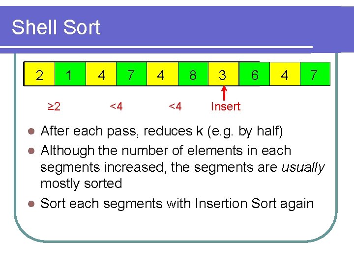
Shell Sort 2 1 ≥ 2 4 7 <4 4 8 <4 3 6 4 7 Insert After each pass, reduces k (e. g. by half) l Although the number of elements in each segments increased, the segments are usually mostly sorted l Sort each segments with Insertion Sort again l

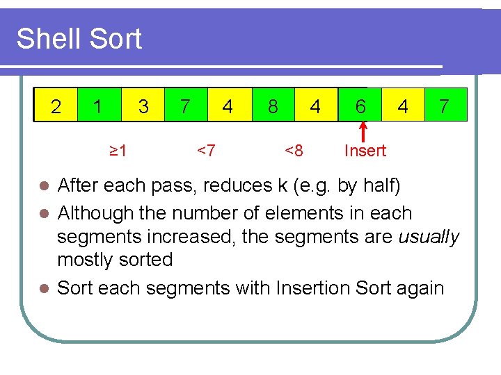
Shell Sort 2 1 3 ≥ 1 7 4 <7 8 4 <8 6 4 7 Insert After each pass, reduces k (e. g. by half) l Although the number of elements in each segments increased, the segments are usually mostly sorted l Sort each segments with Insertion Sort again l

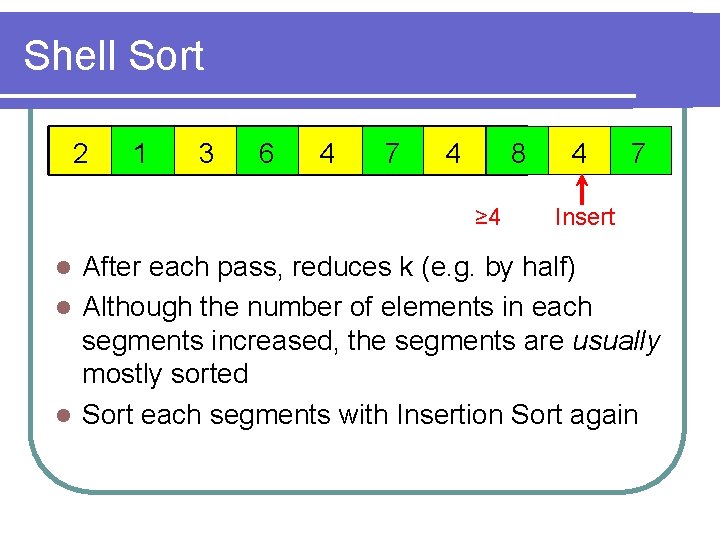
Shell Sort 2 1 3 6 4 7 4 8 ≥ 4 4 7 Insert After each pass, reduces k (e. g. by half) l Although the number of elements in each segments increased, the segments are usually mostly sorted l Sort each segments with Insertion Sort again l

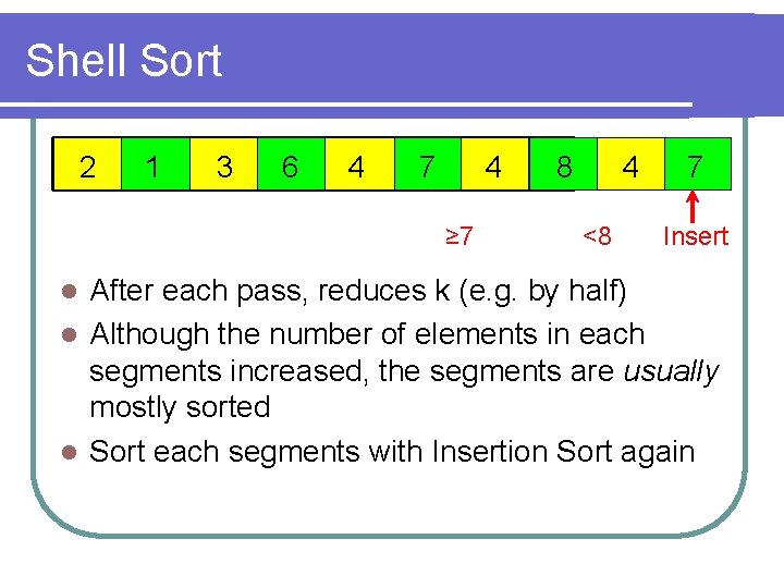
Shell Sort 2 1 3 6 4 7 4 ≥ 7 8 4 <8 7 Insert After each pass, reduces k (e. g. by half) l Although the number of elements in each segments increased, the segments are usually mostly sorted l Sort each segments with Insertion Sort again l

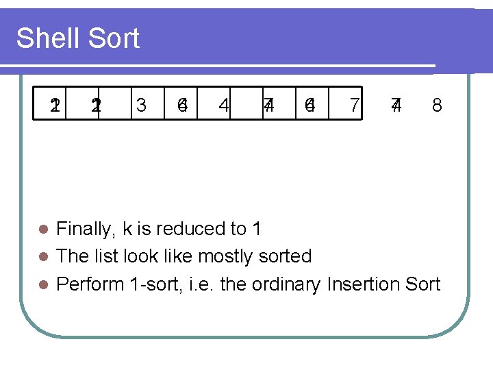
Shell Sort 2 1 1 2 3 6 4 4 7 4 4 6 7 4 7 8 Finally, k is reduced to 1 l The list look like mostly sorted l Perform 1 -sort, i. e. the ordinary Insertion Sort l

Shell Sort – Worse than Ins. Sort? l In Shell Sort, we still have to perform an Insertion Sort at last l A lot of operations are done before the final Insertion Sort l Isn’t it worse than Insertion Sort?

Shell Sort – Worse than Ins. Sort? l The final Insertion Sort is more efficient than before l All sorting operations before the final one are done efficiently l k-sorts compare far-apart elements l Elements “moves” faster, reducing amount of movement and comparison

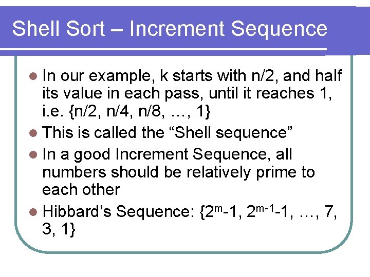
Shell Sort – Increment Sequence l In our example, k starts with n/2, and half its value in each pass, until it reaches 1, i. e. {n/2, n/4, n/8, …, 1} l This is called the “Shell sequence” l In a good Increment Sequence, all numbers should be relatively prime to each other l Hibbard’s Sequence: {2 m-1, 2 m-1 -1, …, 7, 3, 1}

Shell Sort – Analysis l Average Complexity: O(n 1. 5) l Worse case of Shell Sort with Shell Sequence: O(n 2) l When will it happen?

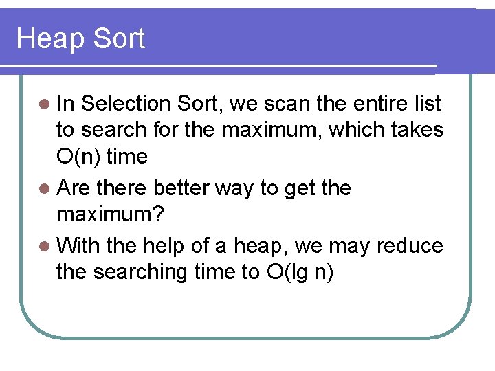
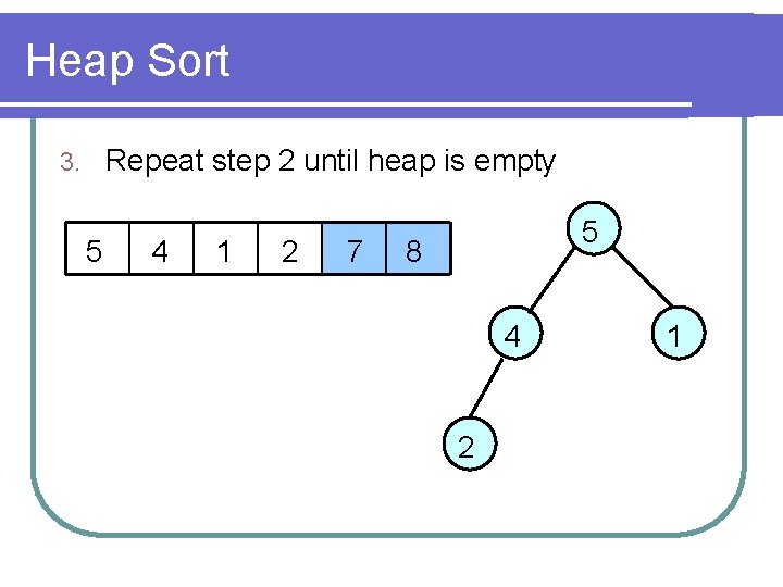
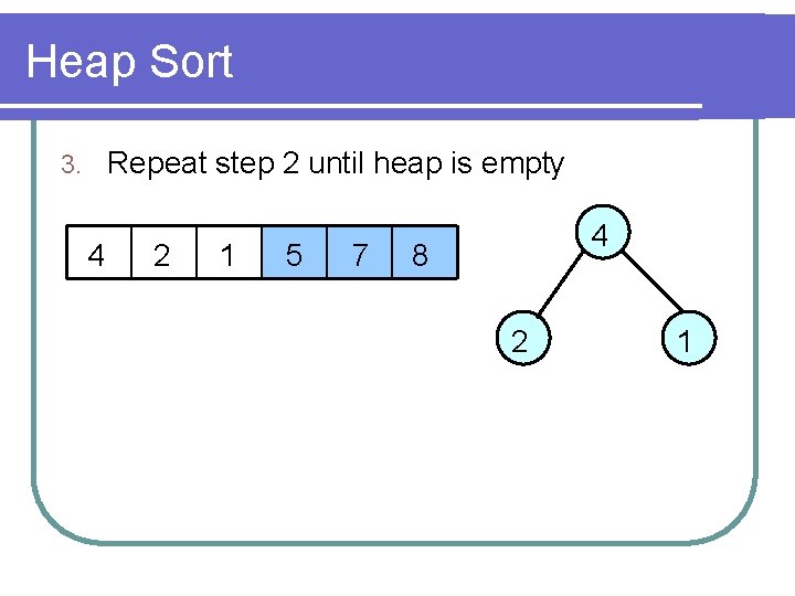
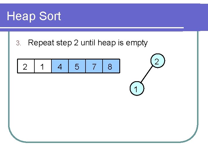
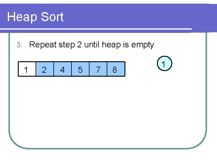
Heap Sort l In Selection Sort, we scan the entire list to search for the maximum, which takes O(n) time l Are there better way to get the maximum? l With the help of a heap, we may reduce the searching time to O(lg n)

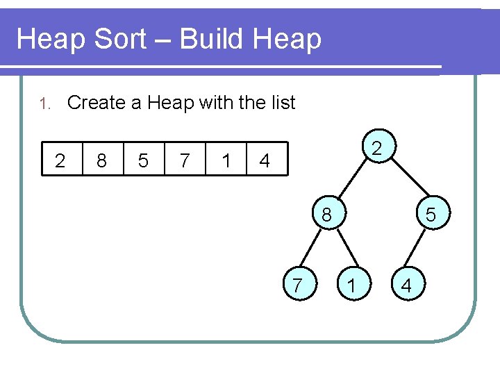
Heap Sort – Build Heap Create a Heap with the list 1. 2 8 5 7 1 2 4 8 7 5 1 4

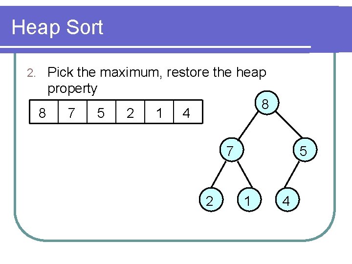
Heap Sort 2. Pick the maximum, restore the heap property 8 8 7 5 2 1 4 7 2 5 1 4

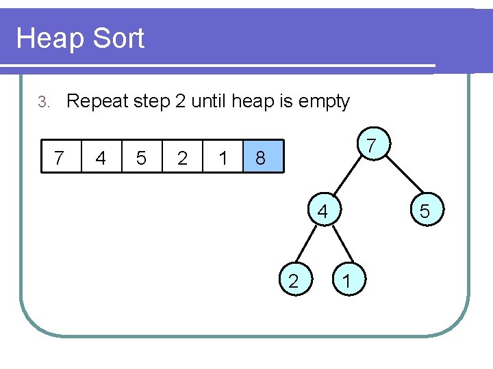
Heap Sort Repeat step 2 until heap is empty 3. 7 4 5 2 1 7 8 4 2 5 1

Heap Sort Repeat step 2 until heap is empty 3. 5 4 1 2 7 5 8 4 2 1

Heap Sort Repeat step 2 until heap is empty 3. 4 2 1 5 7 4 8 2 1

Heap Sort Repeat step 2 until heap is empty 3. 2 1 4 5 7 2 8 1

Heap Sort Repeat step 2 until heap is empty 3. 1 2 4 5 7 8 1

Heap Sort – Analysis l Complexity: O(n lg n) l Not a stable sort l Difficult to implement

Merging l Given two sorted list, merge the list to form a new sorted list l A naïve approach: Append the second list to the first list, then sort them l Slow, takes O(n lg n) time l Are there any better way?

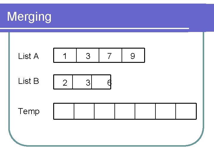
Merging l We make use of a property of sorted lists: The first element is always the minimum l What does that imply? l An additional array is needed store temporary merged list l Pick the smallest number from the uninserted numbers and append them to the merged list

Merging List A 1 3 7 List B 2 3 6 Temp 9

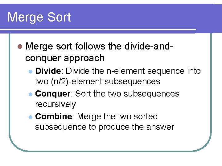
Merge Sort l Merge sort follows the divide-andconquer approach Divide: Divide the n-element sequence into two (n/2)-element subsequences l Conquer: Sort the two subsequences recursively l Combine: Merge the two sorted subsequence to produce the answer l

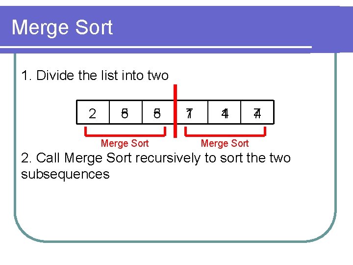
Merge Sort 1. Divide the list into two 2 8 5 Merge Sort 5 8 7 1 1 4 4 7 Merge Sort 2. Call Merge Sort recursively to sort the two subsequences

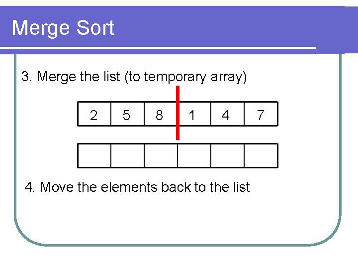
Merge Sort 3. Merge the list (to temporary array) 2 5 8 1 4 4. Move the elements back to the list 7

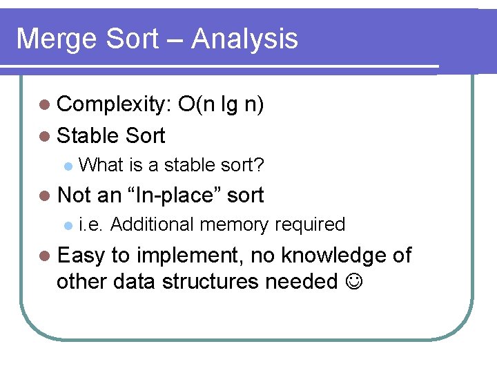
Merge Sort – Analysis l Complexity: l Stable l Sort What is a stable sort? l Not l O(n lg n) an “In-place” sort i. e. Additional memory required l Easy to implement, no knowledge of other data structures needed

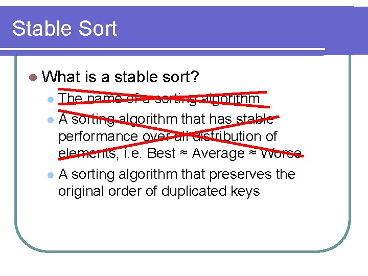
Stable Sort l What is a stable sort? The name of a sorting algorithm l A sorting algorithm that has stable performance over all distribution of elements, i. e. Best ≈ Average ≈ Worse l A sorting algorithm that preserves the original order of duplicated keys l

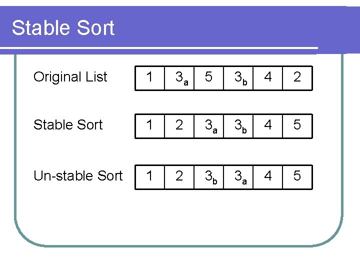
Stable Sort Original List 1 3 a 5 3 b 4 2 Stable Sort 1 2 3 a 3 b 4 5 Un-stable Sort 1 2 3 b 3 a 4 5

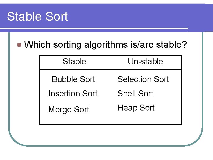
Stable Sort l Which sorting algorithms is/are stable? Stable Un-stable Bubble Sort Selection Sort Insertion Sort Shell Sort Merge Sort Heap Sort

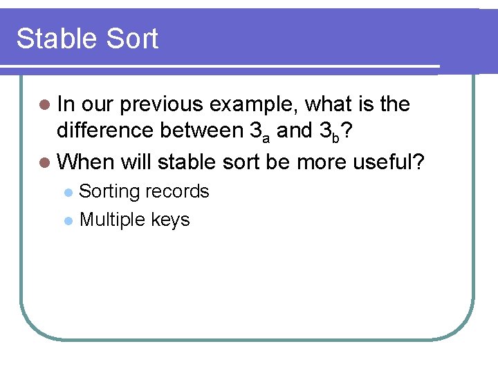
Stable Sort l In our previous example, what is the difference between 3 a and 3 b? l When will stable sort be more useful? Sorting records l Multiple keys l

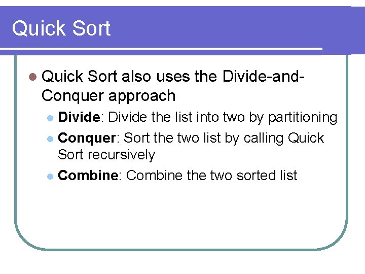
Quick Sort l Quick Sort also uses the Divide-and. Conquer approach Divide: Divide the list into two by partitioning l Conquer: Sort the two list by calling Quick Sort recursively l Combine: Combine the two sorted list l

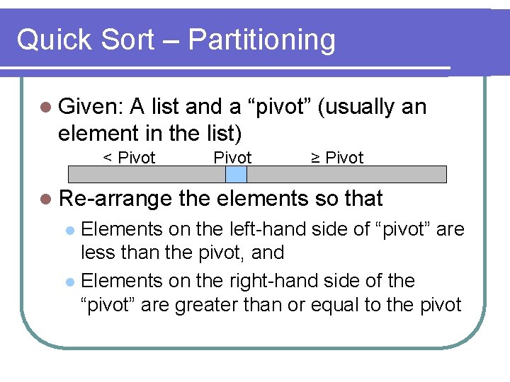
Quick Sort – Partitioning l Given: A list and a “pivot” (usually an element in the list) < Pivot l Re-arrange Pivot ≥ Pivot the elements so that Elements on the left-hand side of “pivot” are less than the pivot, and l Elements on the right-hand side of the “pivot” are greater than or equal to the pivot l

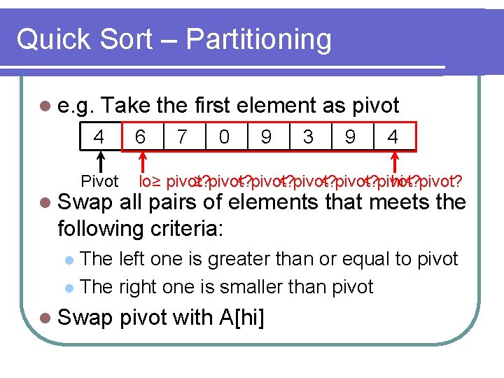
Quick Sort – Partitioning l e. g. Take the first element as pivot 4 Pivot l Swap 6 7 0 9 3 9 4 lo ≥ pivot? < pivot? hi < pivot? all pairs of elements that meets the following criteria: The left one is greater than or equal to pivot l The right one is smaller than pivot l l Swap pivot with A[hi]

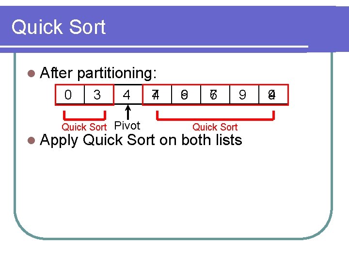
Quick Sort l After partitioning: 0 3 Quick Sort l Apply 4 Pivot 7 4 9 6 6 7 Quick Sort 9 Quick Sort on both lists 4 9

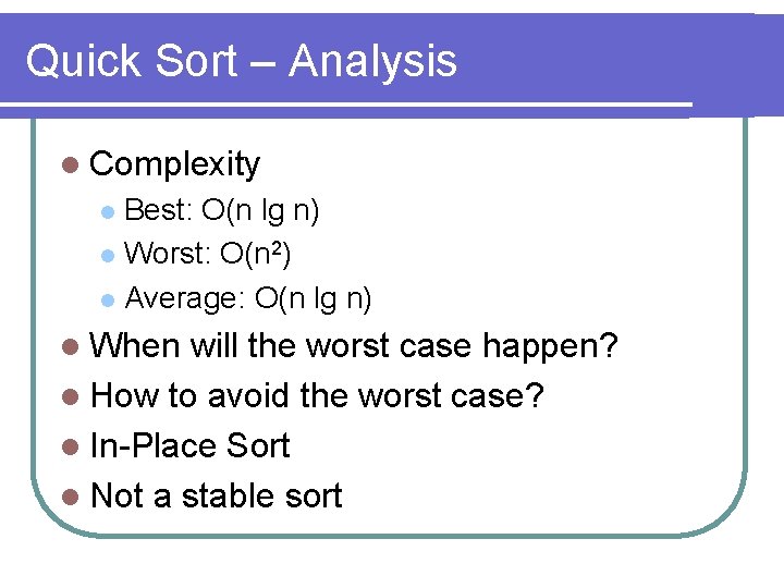
Quick Sort – Analysis l Complexity Best: O(n lg n) l Worst: O(n 2) l Average: O(n lg n) l l When will the worst case happen? l How to avoid the worst case? l In-Place Sort l Not a stable sort

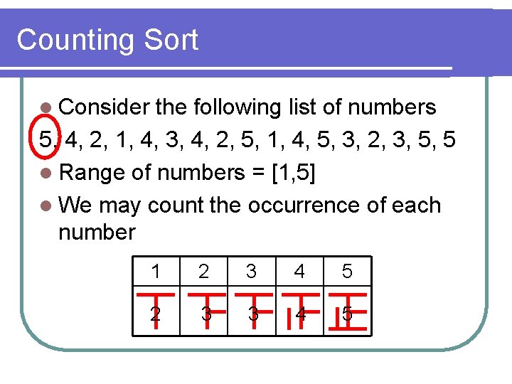
Counting Sort l Consider the following list of numbers 5, 4, 2, 1, 4, 3, 4, 2, 5, 1, 4, 5, 3, 2, 3, 5, 5 l Range of numbers = [1, 5] l We may count the occurrence of each number 1 2 3 4 5 2 3 3 4 5

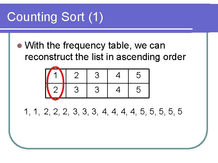
Counting Sort (1) l With the frequency table, we can reconstruct the list in ascending order 1 2 3 4 5 2 3 3 4 5 1, 1, 2, 2, 2, 3, 3, 3, 4, 4, 5, 5, 5

Counting Sort (1) l Can we sort records with this counting sort? l Is this sort stable?

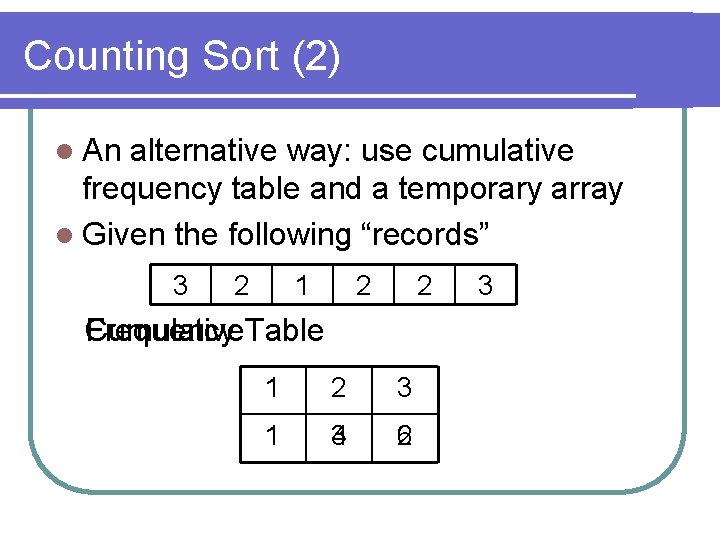
Counting Sort (2) l An alternative way: use cumulative frequency table and a temporary array l Given the following “records” 3 2 1 2 2 Frequency Table Cumulative 1 2 3 1 3 4 2 6 3

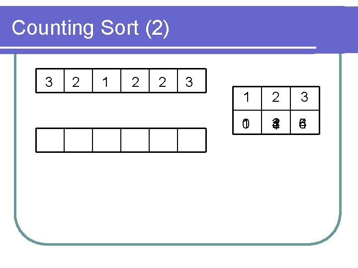
Counting Sort (2) 3 2 1 2 2 3 1 0 2 3 4 1 6 5 4

Counting Sort – Analysis l Complexity: O(n+k), where k is the range of numbers l Not an In-place sort l Stable Sort (Method 2) l Cannot be applied on data with wide ranges

Radix Sort l Counting Sort requires a “frequency table” l The size of frequency table depends on the range of elements l If the range is large (e. g. 32 -bit), it may be infeasible, if not impossible, to create such a table

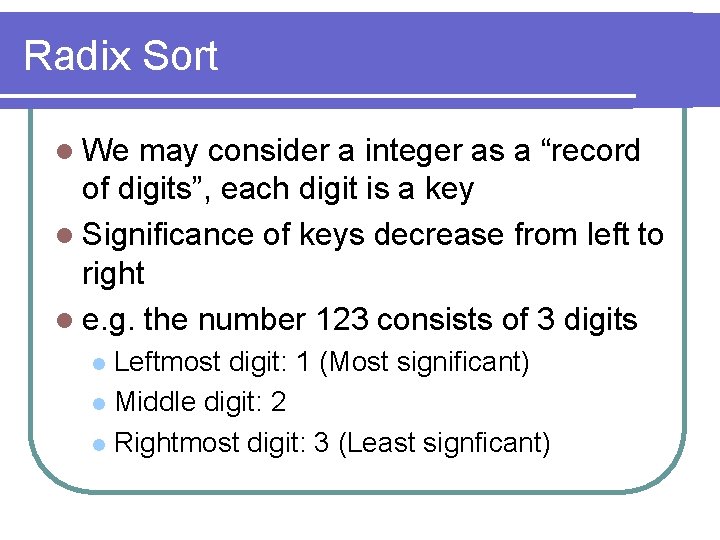
Radix Sort l We may consider a integer as a “record of digits”, each digit is a key l Significance of keys decrease from left to right l e. g. the number 123 consists of 3 digits Leftmost digit: 1 (Most significant) l Middle digit: 2 l Rightmost digit: 3 (Least signficant) l

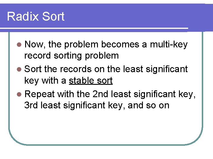
Radix Sort l Now, the problem becomes a multi-key record sorting problem l Sort the records on the least significant key with a stable sort l Repeat with the 2 nd least significant key, 3 rd least significant key, and so on

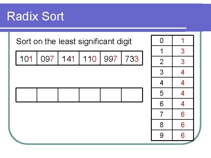
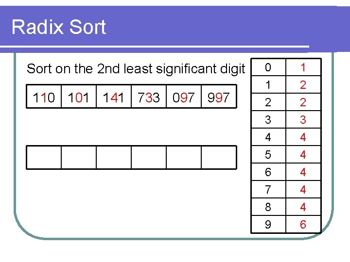
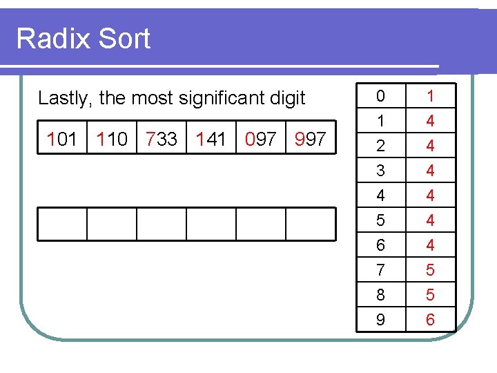
Radix Sort l For all keys in these “records”, the range is [0, 9] Narrow range l We apply Counting Sort to do the sorting here

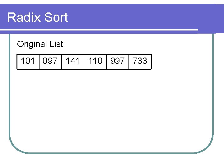
Radix Sort Original List 101 0 97 141 110 997 733

Radix Sort on the least significant digit 101 097 141 110 997 733 0 1 2 3 1 3 3 4 4 5 6 7 8 9 4 4 4 6 6 6

Radix Sort on the 2 nd least significant digit 110 101 141 733 097 997 0 1 2 3 1 2 2 3 4 5 6 7 8 9 4 4 4 6

Radix Sort Lastly, the most significant digit 101 110 733 141 097 997 0 1 2 3 1 4 4 5 6 7 8 9 4 4 4 5 5 6

Radix Sort – Analysis l Complexity: O(dn), where d is the number of digits l Not an In-place Sort l Stable Sort l Can we run Radix Sort on Real numbers? l String? l

Choosing Sorting Algorithms l List Size l Data distribution l Data Type l Availability of Additional Memory l Cost of Swapping/Assignment

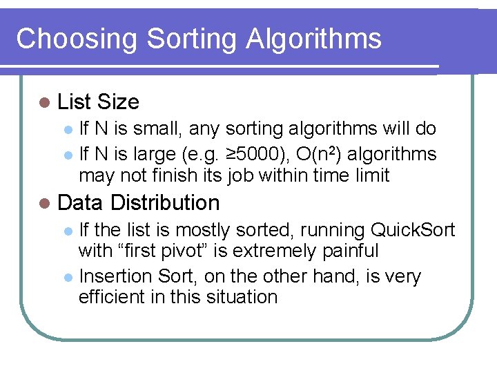
Choosing Sorting Algorithms l List Size If N is small, any sorting algorithms will do l If N is large (e. g. ≥ 5000), O(n 2) algorithms may not finish its job within time limit l l Data Distribution If the list is mostly sorted, running Quick. Sort with “first pivot” is extremely painful l Insertion Sort, on the other hand, is very efficient in this situation l

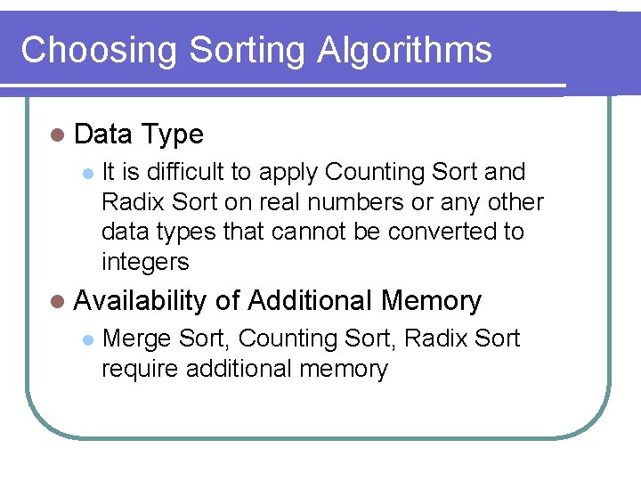
Choosing Sorting Algorithms l Data l Type It is difficult to apply Counting Sort and Radix Sort on real numbers or any other data types that cannot be converted to integers l Availability l of Additional Memory Merge Sort, Counting Sort, Radix Sort require additional memory

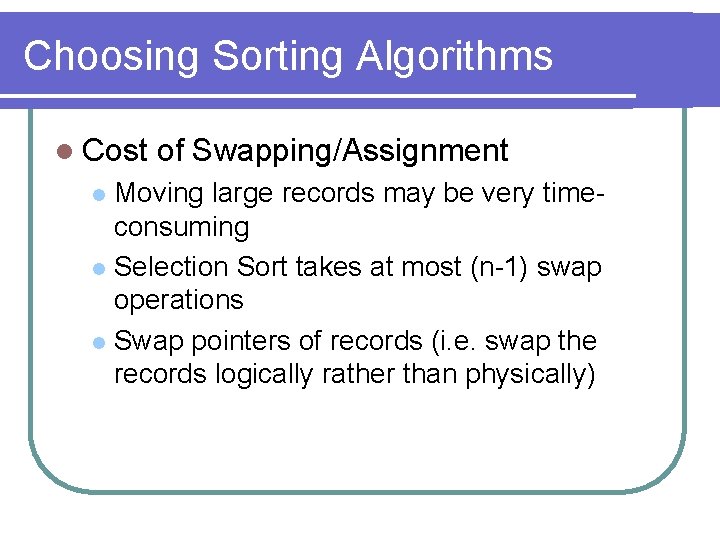
Choosing Sorting Algorithms l Cost of Swapping/Assignment Moving large records may be very timeconsuming l Selection Sort takes at most (n-1) swap operations l Swap pointers of records (i. e. swap the records logically rather than physically) l