Sorting Algorithms Sorting Sorting is a process that
![Selection Sort (cont. ) template <class Item> void selection. Sort( Item a[], int n) Selection Sort (cont. ) template <class Item> void selection. Sort( Item a[], int n)](https://slidetodoc.com/presentation_image/19a2c4e7d5304ab8fde50954abcb5940/image-6.jpg)
![Insertion Sort Algorithm template <class Item> void insertion. Sort(Item a[], int n) { for Insertion Sort Algorithm template <class Item> void insertion. Sort(Item a[], int n) { for](https://slidetodoc.com/presentation_image/19a2c4e7d5304ab8fde50954abcb5940/image-12.jpg)
![Bubble Sort Algorithm template <class Item> void buble. Sort(Item a[], int n) { bool Bubble Sort Algorithm template <class Item> void buble. Sort(Item a[], int n) { bool](https://slidetodoc.com/presentation_image/19a2c4e7d5304ab8fde50954abcb5940/image-17.jpg)
![Merge const int MAX_SIZE = maximum-number-of-items-in-array; void merge(Data. Type the. Array[], int first, int Merge const int MAX_SIZE = maximum-number-of-items-in-array; void merge(Data. Type the. Array[], int first, int](https://slidetodoc.com/presentation_image/19a2c4e7d5304ab8fde50954abcb5940/image-21.jpg)
![Mergesort void mergesort(Data. Type the. Array[], int first, int last) { if (first < Mergesort void mergesort(Data. Type the. Array[], int first, int last) { if (first <](https://slidetodoc.com/presentation_image/19a2c4e7d5304ab8fde50954abcb5940/image-23.jpg)
![Partition Function template <class Data. Type> void partition(Data. Type the. Array[], int first, int Partition Function template <class Data. Type> void partition(Data. Type the. Array[], int first, int](https://slidetodoc.com/presentation_image/19a2c4e7d5304ab8fde50954abcb5940/image-36.jpg)
![Partition Function (cont. ) Moving the. Array[first. Unknown] into S 1 by swapping it Partition Function (cont. ) Moving the. Array[first. Unknown] into S 1 by swapping it](https://slidetodoc.com/presentation_image/19a2c4e7d5304ab8fde50954abcb5940/image-40.jpg)
![Partition Function (cont. ) Moving the. Array[first. Unknown] into S 2 by incrementing first. Partition Function (cont. ) Moving the. Array[first. Unknown] into S 2 by incrementing first.](https://slidetodoc.com/presentation_image/19a2c4e7d5304ab8fde50954abcb5940/image-41.jpg)
![Quicksort Function void quicksort(Data. Type the. Array[], int first, int last) { // Sorts Quicksort Function void quicksort(Data. Type the. Array[], int first, int last) { // Sorts](https://slidetodoc.com/presentation_image/19a2c4e7d5304ab8fde50954abcb5940/image-43.jpg)
- Slides: 53

Sorting Algorithms

Sorting • Sorting is a process that organizes a collection of data into either ascending or descending order. • An internal sort requires that the collection of data fit entirely in the computer’s main memory. • We can use an external sort when the collection of data cannot fit in the computer’s main memory all at once but must reside in secondary storage such as on a disk. • We will analyze only internal sorting algorithms. • Any significant amount of computer output is generally arranged in some sorted order so that it can be interpreted. • Sorting also has indirect uses. An initial sort of the data can significantly enhance the performance of an algorithm. • Majority of programming projects use a sort somewhere, and in many cases, the sorting cost determines the running time. • A comparison-based sorting algorithm makes ordering decisions only on the basis of comparisons.

Sorting Algorithms • There are many sorting algorithms, such as: – Selection Sort – Insertion Sort – Bubble Sort – Merge Sort – Quick Sort • The first three are the foundations for faster and more efficient algorithms.

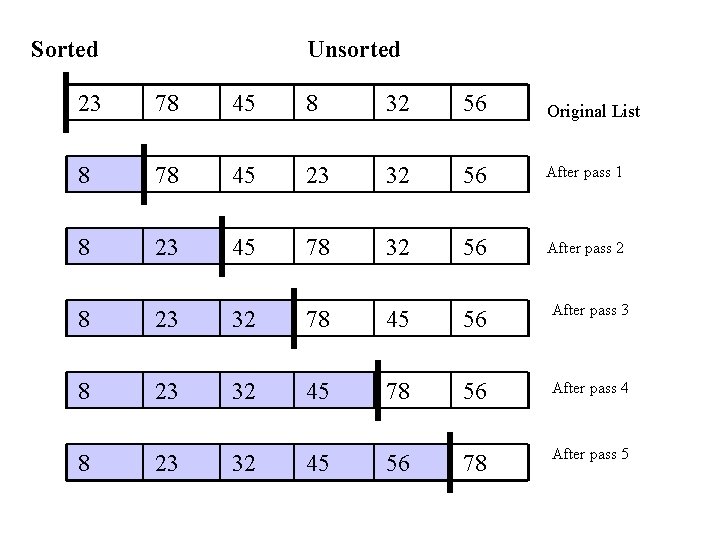
Selection Sort • The list is divided into two sublists, sorted and unsorted, which are divided by an imaginary wall. • We find the smallest element from the unsorted sublist and swap it with the element at the beginning of the unsorted data. • After each selection and swapping, the imaginary wall between the two sublists move one element ahead, increasing the number of sorted elements and decreasing the number of unsorted ones. • Each time we move one element from the unsorted sublist to the sorted sublist, we say that we have completed a sort pass. • A list of n elements requires n-1 passes to completely rearrange the data.

Sorted Unsorted 23 78 45 8 32 56 Original List 8 78 45 23 32 56 After pass 1 8 23 45 78 32 56 After pass 2 8 23 32 78 45 56 After pass 3 8 23 32 45 78 56 After pass 4 8 23 32 45 56 78 After pass 5
![Selection Sort cont template class Item void selection Sort Item a int n Selection Sort (cont. ) template <class Item> void selection. Sort( Item a[], int n)](https://slidetodoc.com/presentation_image/19a2c4e7d5304ab8fde50954abcb5940/image-6.jpg)
Selection Sort (cont. ) template <class Item> void selection. Sort( Item a[], int n) { for (int i = 0; i < n-1; i++) { int min = i; for (int j = i+1; j < n; j++) if (a[j] < a[min]) min = j; swap(a[i], a[min]); } } template < class Object> void swap( Object &lhs, Object &rhs ) { Object tmp = lhs; lhs = rhs; rhs = tmp; }

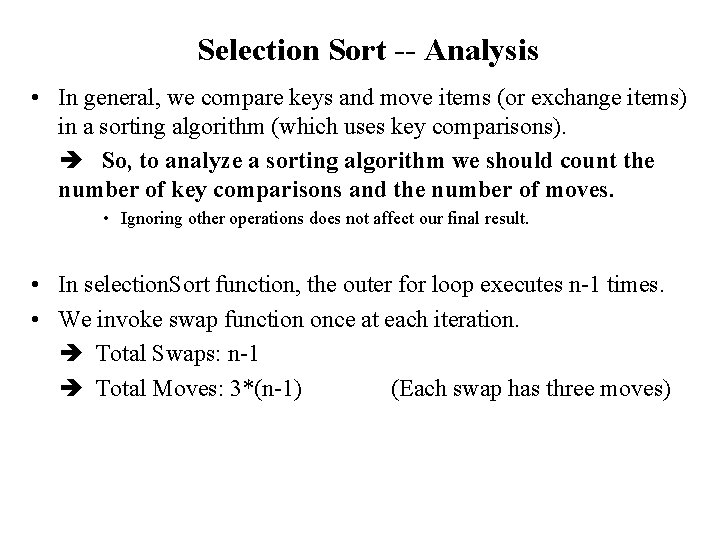
Selection Sort -- Analysis • In general, we compare keys and move items (or exchange items) in a sorting algorithm (which uses key comparisons). So, to analyze a sorting algorithm we should count the number of key comparisons and the number of moves. • Ignoring other operations does not affect our final result. • In selection. Sort function, the outer for loop executes n-1 times. • We invoke swap function once at each iteration. Total Swaps: n-1 Total Moves: 3*(n-1) (Each swap has three moves)

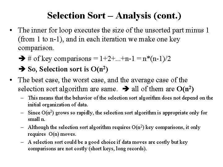
Selection Sort – Analysis (cont. ) • The inner for loop executes the size of the unsorted part minus 1 (from 1 to n-1), and in each iteration we make one key comparison. # of key comparisons = 1+2+. . . +n-1 = n*(n-1)/2 So, Selection sort is O(n 2) • The best case, the worst case, and the average case of the selection sort algorithm are same. all of them are O(n 2) – This means that the behavior of the selection sort algorithm does not depend on the initial organization of data. – Since O(n 2) grows so rapidly, the selection sort algorithm is appropriate only for small n. – Although the selection sort algorithm requires O(n 2) key comparisons, it only requires O(n) moves. – A selection sort could be a good choice if data moves are costly but key comparisons are not costly (short keys, long records).

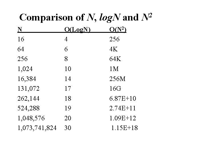
Comparison of N, log. N and N 2 N 16 64 256 1, 024 16, 384 131, 072 262, 144 524, 288 1, 048, 576 1, 073, 741, 824 O(Log. N) 4 6 8 10 14 17 18 19 20 30 O(N 2) 256 4 K 64 K 1 M 256 M 16 G 6. 87 E+10 2. 74 E+11 1. 09 E+12 1. 15 E+18

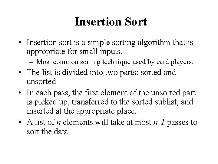
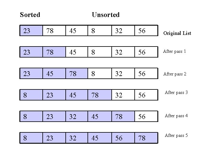
Insertion Sort • Insertion sort is a simple sorting algorithm that is appropriate for small inputs. – Most common sorting technique used by card players. • The list is divided into two parts: sorted and unsorted. • In each pass, the first element of the unsorted part is picked up, transferred to the sorted sublist, and inserted at the appropriate place. • A list of n elements will take at most n-1 passes to sort the data.

Sorted Unsorted 23 78 45 8 32 56 Original List 23 78 45 8 32 56 After pass 1 23 45 78 8 32 56 After pass 2 8 23 45 78 32 56 After pass 3 8 23 32 45 78 56 After pass 4 8 23 32 45 56 78 After pass 5
![Insertion Sort Algorithm template class Item void insertion SortItem a int n for Insertion Sort Algorithm template <class Item> void insertion. Sort(Item a[], int n) { for](https://slidetodoc.com/presentation_image/19a2c4e7d5304ab8fde50954abcb5940/image-12.jpg)
Insertion Sort Algorithm template <class Item> void insertion. Sort(Item a[], int n) { for (int i = 1; i < n; i++) { Item tmp = a[i]; for (int j=i; j>0 && tmp < a[j-1]; j--) a[j] = a[j-1]; a[j] = tmp; } }

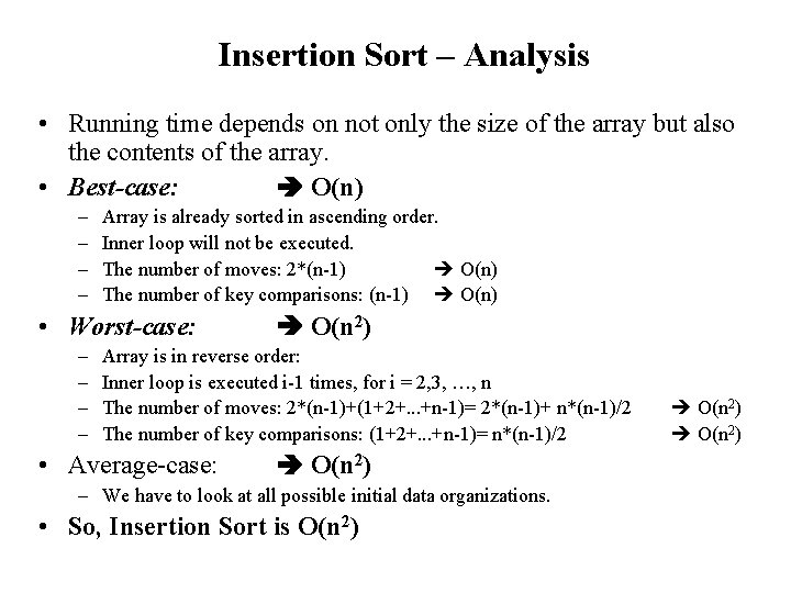
Insertion Sort – Analysis • Running time depends on not only the size of the array but also the contents of the array. • Best-case: O(n) – – Array is already sorted in ascending order. Inner loop will not be executed. The number of moves: 2*(n-1) O(n) The number of key comparisons: (n-1) O(n) • Worst-case: – – O(n 2) Array is in reverse order: Inner loop is executed i-1 times, for i = 2, 3, …, n The number of moves: 2*(n-1)+(1+2+. . . +n-1)= 2*(n-1)+ n*(n-1)/2 The number of key comparisons: (1+2+. . . +n-1)= n*(n-1)/2 • Average-case: O(n 2) – We have to look at all possible initial data organizations. • So, Insertion Sort is O(n 2)

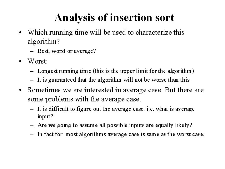
Analysis of insertion sort • Which running time will be used to characterize this algorithm? – Best, worst or average? • Worst: – Longest running time (this is the upper limit for the algorithm) – It is guaranteed that the algorithm will not be worse than this. • Sometimes we are interested in average case. But there are some problems with the average case. – It is difficult to figure out the average case. i. e. what is average input? – Are we going to assume all possible inputs are equally likely? – In fact for most algorithms average case is same as the worst case.

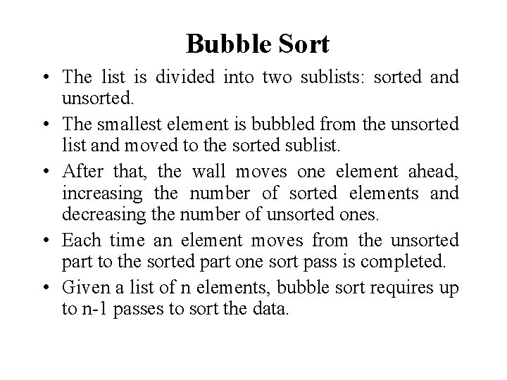
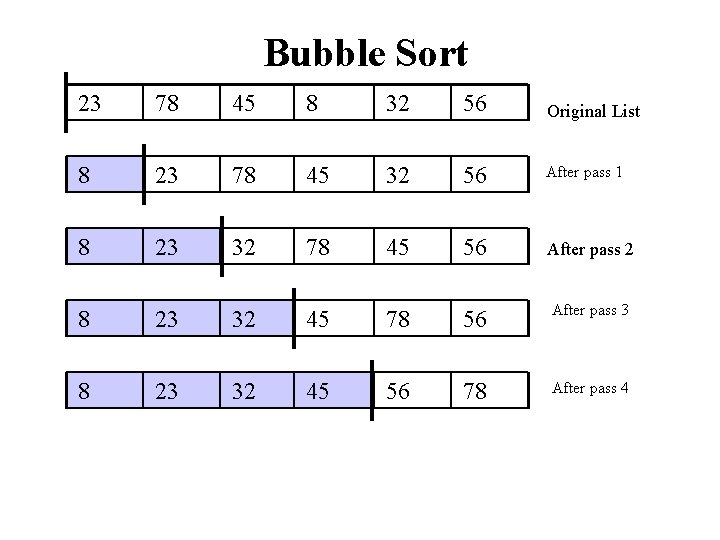
Bubble Sort • The list is divided into two sublists: sorted and unsorted. • The smallest element is bubbled from the unsorted list and moved to the sorted sublist. • After that, the wall moves one element ahead, increasing the number of sorted elements and decreasing the number of unsorted ones. • Each time an element moves from the unsorted part to the sorted part one sort pass is completed. • Given a list of n elements, bubble sort requires up to n-1 passes to sort the data.

Bubble Sort 23 78 45 8 32 56 Original List 8 23 78 45 32 56 After pass 1 8 23 32 78 45 56 After pass 2 8 23 32 45 78 56 After pass 3 8 23 32 45 56 78 After pass 4
![Bubble Sort Algorithm template class Item void buble SortItem a int n bool Bubble Sort Algorithm template <class Item> void buble. Sort(Item a[], int n) { bool](https://slidetodoc.com/presentation_image/19a2c4e7d5304ab8fde50954abcb5940/image-17.jpg)
Bubble Sort Algorithm template <class Item> void buble. Sort(Item a[], int n) { bool sorted = false; int last = n-1; for (int i = 0; (i < last) && !sorted; i++){ sorted = true; for (int j=last; j > i; j--) if (a[j-1] > a[j]{ swap(a[j], a[j-1]); sorted = false; // signal exchange } } }

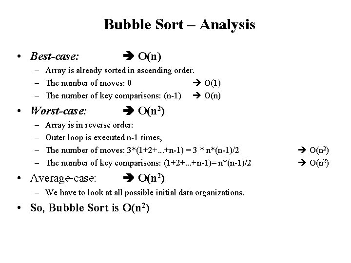
Bubble Sort – Analysis • Best-case: O(n) – Array is already sorted in ascending order. – The number of moves: 0 O(1) – The number of key comparisons: (n-1) O(n) • Worst-case: – – O(n 2) Array is in reverse order: Outer loop is executed n-1 times, The number of moves: 3*(1+2+. . . +n-1) = 3 * n*(n-1)/2 The number of key comparisons: (1+2+. . . +n-1)= n*(n-1)/2 • Average-case: O(n 2) – We have to look at all possible initial data organizations. • So, Bubble Sort is O(n 2)

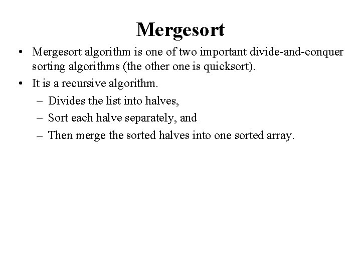
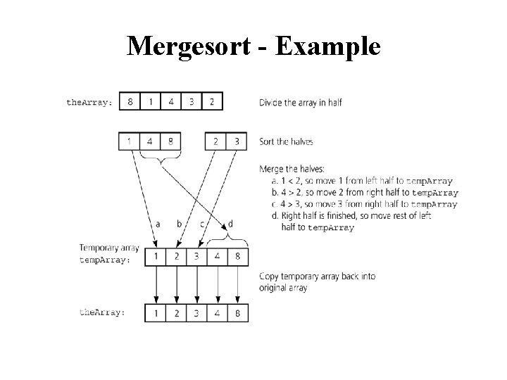
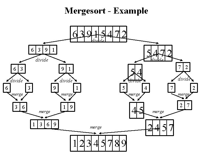
Mergesort • Mergesort algorithm is one of two important divide-and-conquer sorting algorithms (the other one is quicksort). • It is a recursive algorithm. – Divides the list into halves, – Sort each halve separately, and – Then merge the sorted halves into one sorted array.

Mergesort - Example
![Merge const int MAXSIZE maximumnumberofitemsinarray void mergeData Type the Array int first int Merge const int MAX_SIZE = maximum-number-of-items-in-array; void merge(Data. Type the. Array[], int first, int](https://slidetodoc.com/presentation_image/19a2c4e7d5304ab8fde50954abcb5940/image-21.jpg)
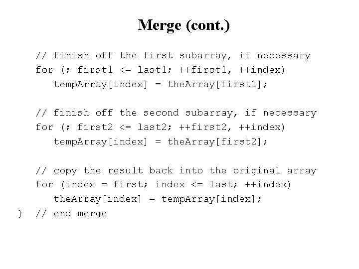
Merge const int MAX_SIZE = maximum-number-of-items-in-array; void merge(Data. Type the. Array[], int first, int mid, int last) { Data. Type temp. Array[MAX_SIZE]; // temporary array int first 1 = first; // beginning of first subarray int last 1 = mid; // end of first subarray int first 2 = mid + 1; // beginning of second subarray int last 2 = last; // end of second subarray int index = first 1; // next available location in temp. Array for ( ; (first 1 <= last 1) && (first 2 <= last 2); ++index) { if (the. Array[first 1] < the. Array[first 2]) { temp. Array[index] = the. Array[first 1]; ++first 1; } else { temp. Array[index] = the. Array[first 2]; ++first 2; } }

Merge (cont. ) // finish off the first subarray, if necessary for (; first 1 <= last 1; ++first 1, ++index) temp. Array[index] = the. Array[first 1]; // finish off the second subarray, if necessary for (; first 2 <= last 2; ++first 2, ++index) temp. Array[index] = the. Array[first 2]; } // copy the result back into the original array for (index = first; index <= last; ++index) the. Array[index] = temp. Array[index]; // end merge
![Mergesort void mergesortData Type the Array int first int last if first Mergesort void mergesort(Data. Type the. Array[], int first, int last) { if (first <](https://slidetodoc.com/presentation_image/19a2c4e7d5304ab8fde50954abcb5940/image-23.jpg)
Mergesort void mergesort(Data. Type the. Array[], int first, int last) { if (first < last) { int mid = (first + last)/2; // index of midpoint mergesort(the. Array, first, mid); mergesort(the. Array, mid+1, last); // merge the two halves merge(the. Array, first, mid, last); } } // end mergesort

Mergesort - Example 6 3 9 divide 15472 6 3 9 1 5 divide 472 divide 6 3 9 1 divide 6 3 3 6 54 1 5 merge 1 3 6 9 divide 9 merge 7 2 4 7 merge 1 9 45 merge 12345789 2 merge 2 7 merge 2457

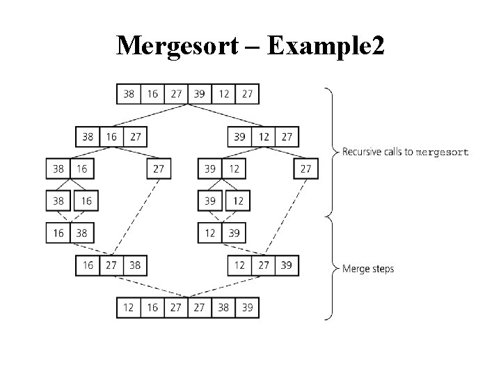
Mergesort – Example 2

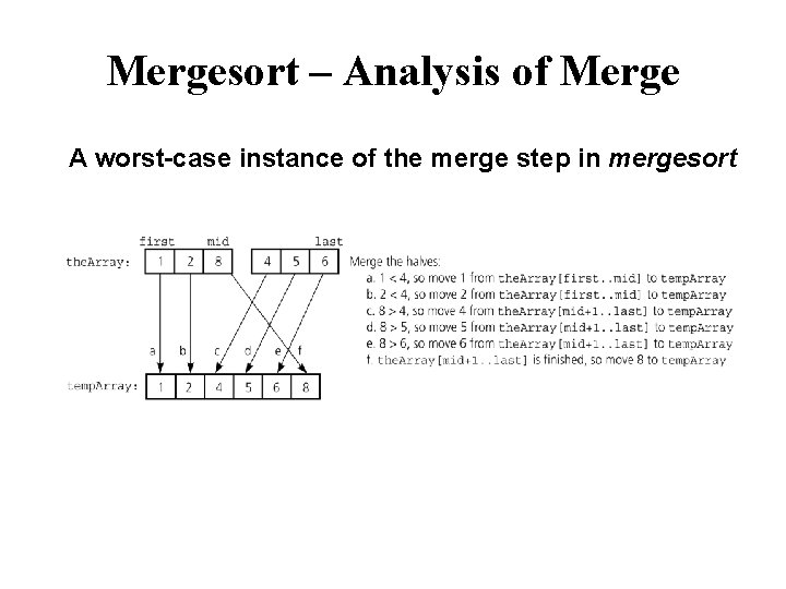
Mergesort – Analysis of Merge A worst-case instance of the merge step in mergesort

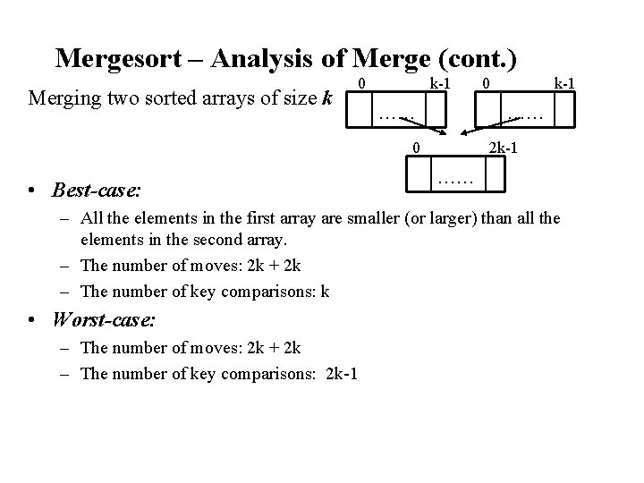
Mergesort – Analysis of Merge (cont. ) Merging two sorted arrays of size k 0 k-1 . . . 0 2 k-1 • Best-case: . . . – All the elements in the first array are smaller (or larger) than all the elements in the second array. – The number of moves: 2 k + 2 k – The number of key comparisons: k • Worst-case: – The number of moves: 2 k + 2 k – The number of key comparisons: 2 k-1

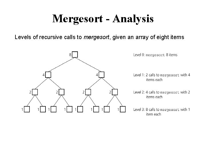
Mergesort - Analysis Levels of recursive calls to mergesort, given an array of eight items

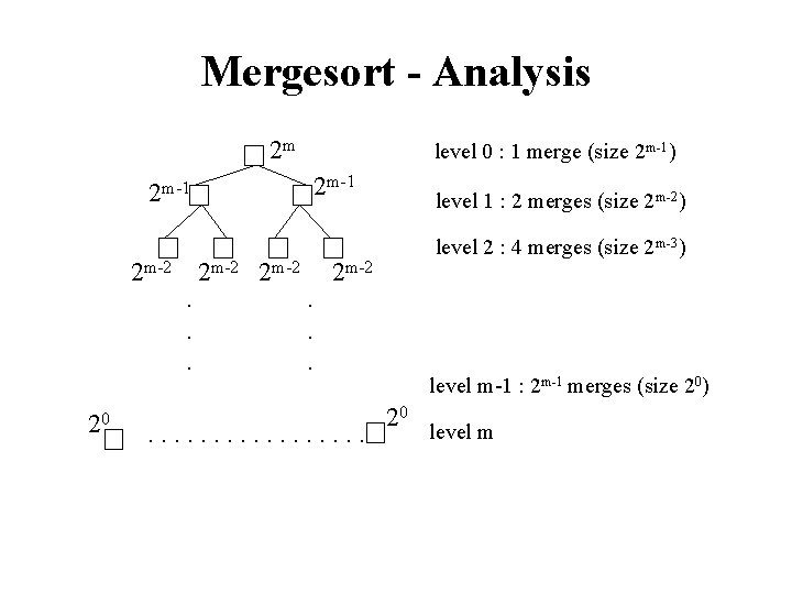
Mergesort - Analysis 2 m 2 m-1 level 0 : 1 merge (size 2 m-1) 2 m-1 level 1 : 2 merges (size 2 m-2) level 2 : 4 merges (size 2 m-3) 2 m-2. . . 20 . . . . level m-1 : 2 m-1 merges (size 20) 20 level m

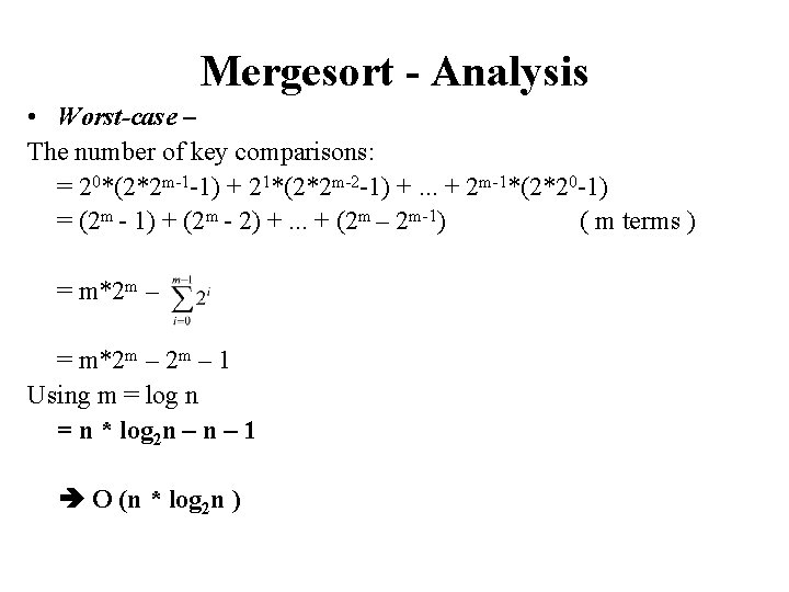
Mergesort - Analysis • Worst-case – The number of key comparisons: = 20*(2*2 m-1 -1) + 21*(2*2 m-2 -1) +. . . + 2 m-1*(2*20 -1) = (2 m - 1) + (2 m - 2) +. . . + (2 m – 2 m-1) ( m terms ) = m*2 m – 1 Using m = log n = n * log 2 n – 1 O (n * log 2 n )

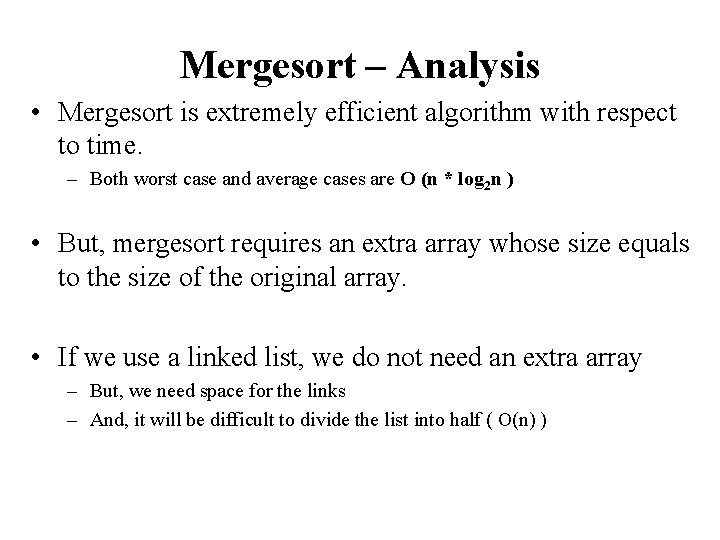
Mergesort – Analysis • Mergesort is extremely efficient algorithm with respect to time. – Both worst case and average cases are O (n * log 2 n ) • But, mergesort requires an extra array whose size equals to the size of the original array. • If we use a linked list, we do not need an extra array – But, we need space for the links – And, it will be difficult to divide the list into half ( O(n) )

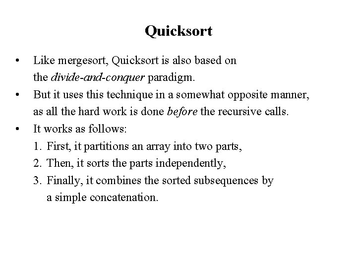
Quicksort • • • Like mergesort, Quicksort is also based on the divide-and-conquer paradigm. But it uses this technique in a somewhat opposite manner, as all the hard work is done before the recursive calls. It works as follows: 1. First, it partitions an array into two parts, 2. Then, it sorts the parts independently, 3. Finally, it combines the sorted subsequences by a simple concatenation.

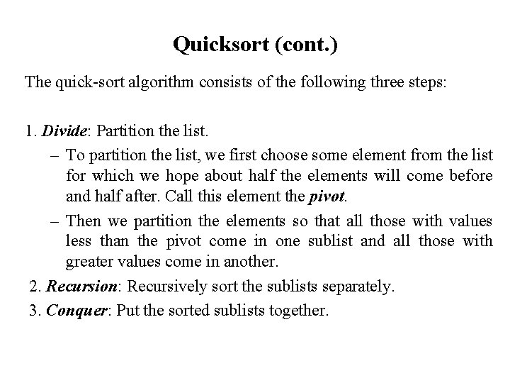
Quicksort (cont. ) The quick-sort algorithm consists of the following three steps: 1. Divide: Partition the list. – To partition the list, we first choose some element from the list for which we hope about half the elements will come before and half after. Call this element the pivot. – Then we partition the elements so that all those with values less than the pivot come in one sublist and all those with greater values come in another. 2. Recursion: Recursively sort the sublists separately. 3. Conquer: Put the sorted sublists together.

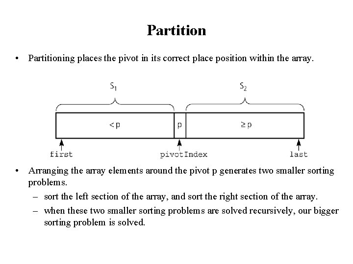
Partition • Partitioning places the pivot in its correct place position within the array. • Arranging the array elements around the pivot p generates two smaller sorting problems. – sort the left section of the array, and sort the right section of the array. – when these two smaller sorting problems are solved recursively, our bigger sorting problem is solved.

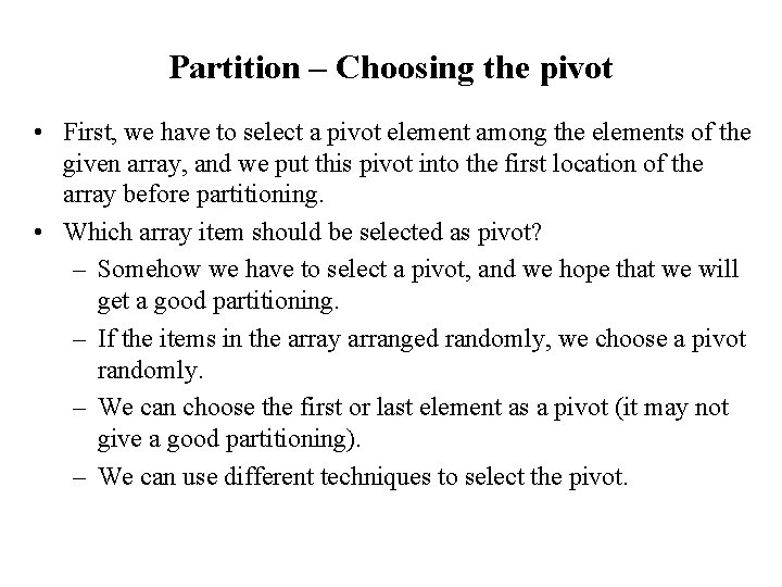
Partition – Choosing the pivot • First, we have to select a pivot element among the elements of the given array, and we put this pivot into the first location of the array before partitioning. • Which array item should be selected as pivot? – Somehow we have to select a pivot, and we hope that we will get a good partitioning. – If the items in the array arranged randomly, we choose a pivot randomly. – We can choose the first or last element as a pivot (it may not give a good partitioning). – We can use different techniques to select the pivot.
![Partition Function template class Data Type void partitionData Type the Array int first int Partition Function template <class Data. Type> void partition(Data. Type the. Array[], int first, int](https://slidetodoc.com/presentation_image/19a2c4e7d5304ab8fde50954abcb5940/image-36.jpg)
Partition Function template <class Data. Type> void partition(Data. Type the. Array[], int first, int last, int &pivot. Index) { // Partitions an array for quicksort. // Precondition: first <= last. // Postcondition: Partitions the. Array[first. . last] such that: // S 1 = the. Array[first. . pivot. Index-1] < pivot // the. Array[pivot. Index] == pivot // S 2 = the. Array[pivot. Index+1. . last] >= pivot // Calls: choose. Pivot and swap. // place pivot in the. Array[first] choose. Pivot(the. Array, first, last); Data. Type pivot = the. Array[first]; // copy pivot

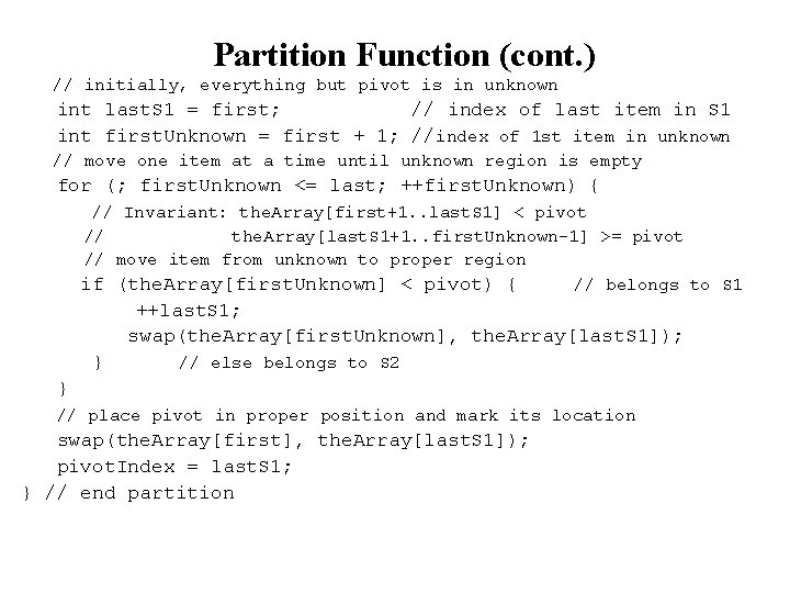
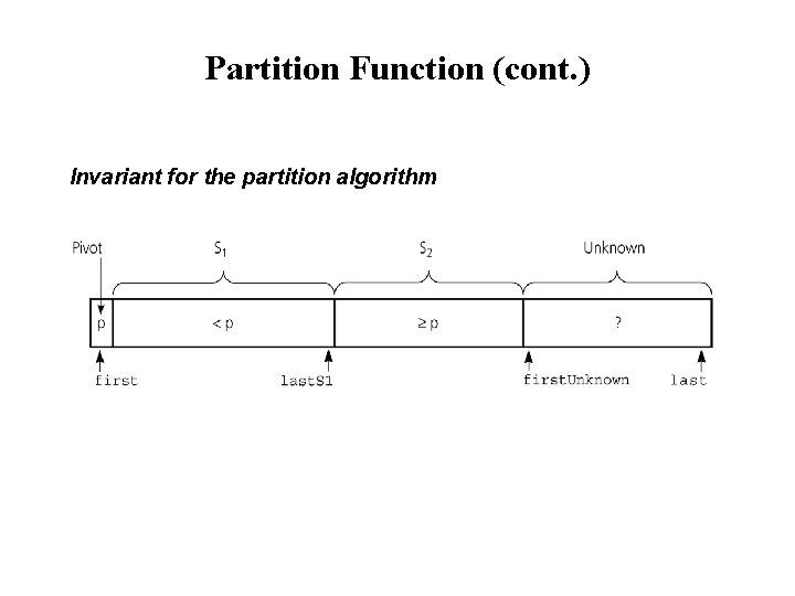
Partition Function (cont. ) // initially, everything but pivot is in unknown int last. S 1 = first; // index of last item in S 1 int first. Unknown = first + 1; //index of 1 st item in unknown // move one item at a time until unknown region is empty for (; first. Unknown <= last; ++first. Unknown) { // Invariant: the. Array[first+1. . last. S 1] < pivot // the. Array[last. S 1+1. . first. Unknown-1] >= pivot // move item from unknown to proper region if (the. Array[first. Unknown] < pivot) { // belongs to S 1 ++last. S 1; swap(the. Array[first. Unknown], the. Array[last. S 1]); } // else belongs to S 2 } // place pivot in proper position and mark its location swap(the. Array[first], the. Array[last. S 1]); pivot. Index = last. S 1; } // end partition

Partition Function (cont. ) Invariant for the partition algorithm

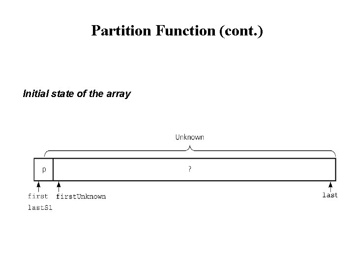
Partition Function (cont. ) Initial state of the array
![Partition Function cont Moving the Arrayfirst Unknown into S 1 by swapping it Partition Function (cont. ) Moving the. Array[first. Unknown] into S 1 by swapping it](https://slidetodoc.com/presentation_image/19a2c4e7d5304ab8fde50954abcb5940/image-40.jpg)
Partition Function (cont. ) Moving the. Array[first. Unknown] into S 1 by swapping it with the. Array[last. S 1+1] and by incrementing both last. S 1 and first. Unknown.
![Partition Function cont Moving the Arrayfirst Unknown into S 2 by incrementing first Partition Function (cont. ) Moving the. Array[first. Unknown] into S 2 by incrementing first.](https://slidetodoc.com/presentation_image/19a2c4e7d5304ab8fde50954abcb5940/image-41.jpg)
Partition Function (cont. ) Moving the. Array[first. Unknown] into S 2 by incrementing first. Unknown.

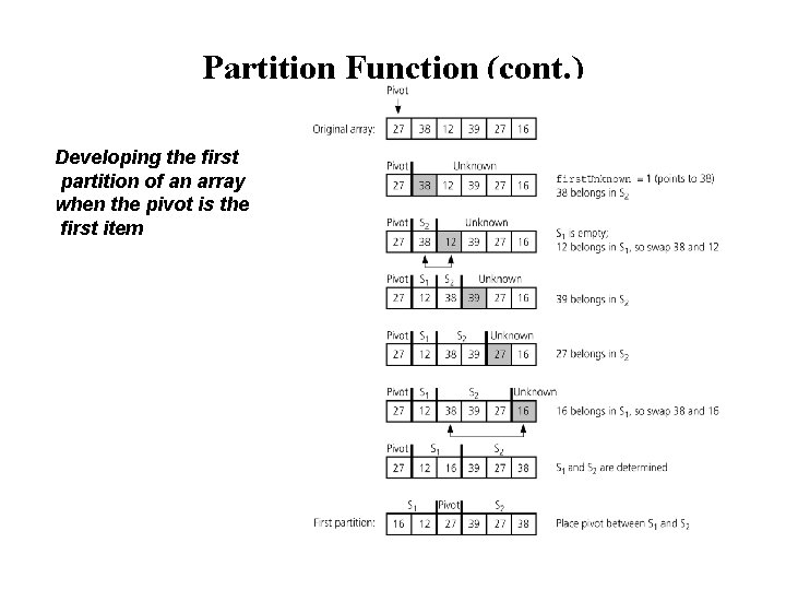
Partition Function (cont. ) Developing the first partition of an array when the pivot is the first item
![Quicksort Function void quicksortData Type the Array int first int last Sorts Quicksort Function void quicksort(Data. Type the. Array[], int first, int last) { // Sorts](https://slidetodoc.com/presentation_image/19a2c4e7d5304ab8fde50954abcb5940/image-43.jpg)
Quicksort Function void quicksort(Data. Type the. Array[], int first, int last) { // Sorts the items in an array into ascending order. // Precondition: the. Array[first. . last] is an array. // Postcondition: the. Array[first. . last] is sorted. // Calls: partition. int pivot. Index; if (first < last) { // create the partition: S 1, pivot, S 2 partition(the. Array, first, last, pivot. Index); // sort regions S 1 and S 2 quicksort(the. Array, first, pivot. Index-1); quicksort(the. Array, pivot. Index+1, last); } }

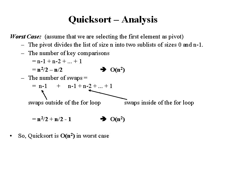
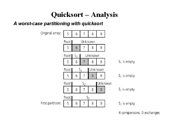
Quicksort – Analysis Worst Case: (assume that we are selecting the first element as pivot) – The pivot divides the list of size n into two sublists of sizes 0 and n-1. – The number of key comparisons = n-1 + n-2 +. . . + 1 = n 2/2 – n/2 O(n 2) – The number of swaps = = n-1 + n-2 +. . . + 1 swaps outside of the for loop = n 2/2 + n/2 - 1 O(n 2) • So, Quicksort is O(n 2) in worst case swaps inside of the for loop

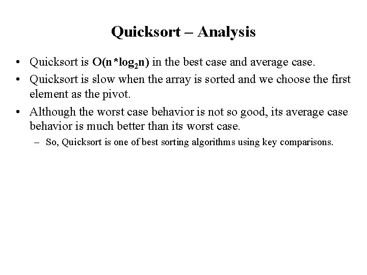
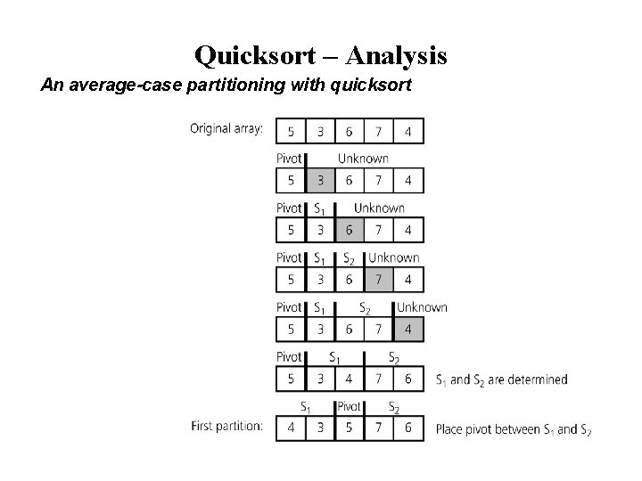
Quicksort – Analysis • Quicksort is O(n*log 2 n) in the best case and average case. • Quicksort is slow when the array is sorted and we choose the first element as the pivot. • Although the worst case behavior is not so good, its average case behavior is much better than its worst case. – So, Quicksort is one of best sorting algorithms using key comparisons.

Quicksort – Analysis A worst-case partitioning with quicksort

Quicksort – Analysis An average-case partitioning with quicksort

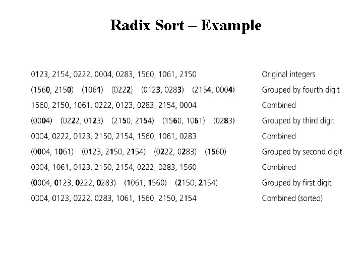
Radix Sort • Radix sort algorithm different than other sorting algorithms that we talked. – It does not use key comparisons to sort an array. • The radix sort : – Treats each data item as a character string. – First it groups data items according to their rightmost character, and put these groups into order w. r. t. this rightmost character. – Then, combine these groups. – We, repeat these grouping and combining operations for all other character positions in the data items from the rightmost to the leftmost character position. – At the end, the sort operation will be completed.

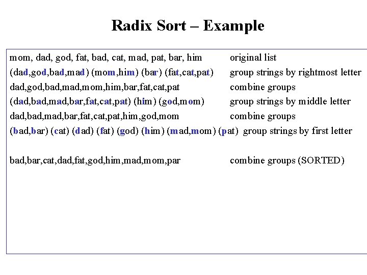
Radix Sort – Example mom, dad, god, fat, bad, cat, mad, pat, bar, him original list (dad, god, bad, mad) (mom, him) (bar) (fat, cat, pat) group strings by rightmost letter dad, god, bad, mom, him, bar, fat, cat, pat combine groups (dad, bad, mad, bar, fat, cat, pat) (him) (god, mom) group strings by middle letter dad, bad, mad, bar, fat, cat, pat, him, god, mom combine groups (bad, bar) (cat) (dad) (fat) (god) (him) (mad, mom) (pat) group strings by first letter bad, bar, cat, dad, fat, god, him, mad, mom, par combine groups (SORTED)

Radix Sort – Example

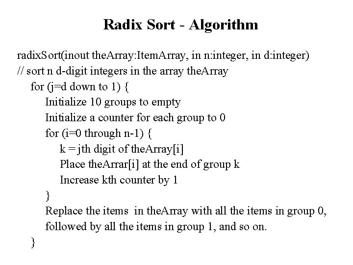
Radix Sort - Algorithm radix. Sort(inout the. Array: Item. Array, in n: integer, in d: integer) // sort n d-digit integers in the array the. Array for (j=d down to 1) { Initialize 10 groups to empty Initialize a counter for each group to 0 for (i=0 through n-1) { k = jth digit of the. Array[i] Place the. Arrar[i] at the end of group k Increase kth counter by 1 } Replace the items in the. Array with all the items in group 0, followed by all the items in group 1, and so on. }

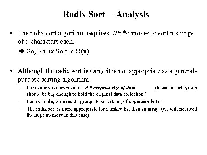
Radix Sort -- Analysis • The radix sort algorithm requires 2*n*d moves to sort n strings of d characters each. So, Radix Sort is O(n) • Although the radix sort is O(n), it is not appropriate as a generalpurpose sorting algorithm. – Its memory requirement is d * original size of data (because each group should be big enough to hold the original data collection. ) – For example, we need 27 groups to sort string of uppercase letters. – The radix sort is more appropriate for a linked list than an array. (we will not need the huge memory in this case)

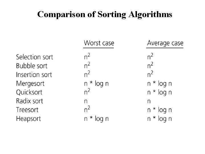
Comparison of Sorting Algorithms