Sorting Recap More about Sorting G C and

Sorting Recap & More about Sorting [G], [C], and [L] Goodrich, Tamassia 1

Bubble sort Details in [L] page 100 Goodrich, Tamassia 2

Bubble sort Details in [L] page 101 Goodrich, Tamassia 3

Selection sort Details in [L] page 99 Goodrich, Tamassia 4

Selection sort Details in [L] page 99 Goodrich, Tamassia 5

Insertion sort Details in [L] page 134 Goodrich, Tamassia 6

Insertion sort Details in [L] page 135 Goodrich, Tamassia 7

New: Shell’s sort Divide the array into smaller subarrays that are “gap” apart Sort subarrays Decrease “gap” Sort again [[ “easier” sort ]] Goodrich, Tamassia 8

9 Shell Sort: A Better Insertion Sort A Shell sort is a type of insertion sort, but with O(n 3/2) or better performance than the O(n 2) sorts It is named after its discoverer, Donald Shell’s sort can be thought of as a divide-andconquer approach to insertion sort Instead of sorting the entire array, Shell sorts many smaller subarrays using insertion sort before sorting the entire array

Subarrays gap = 5 10

Subarrays gap = 2 11

Shell Sort Algorithm 12 Shell Sort Algorithm 1. Set the initial value of gap to n / 2 2. while gap > 0 3. for each array element from position gap to the last element 4. Insert this element where it belongs in its subarray. 5. if gap is 2, set it to 1 6. else gap = gap / 2. 2. // chosen by experimentation

Analysis of Shell Sort 13 Because the behavior of insertion sort is closer to O(n) than O(n 2) when an array is nearly sorted, presorting speeds up later sorting This is critical when sorting large arrays where the O(n 2) performance becomes significant

Analysis of Shell Sort (cont. ) 14 A general analysis of Shell sort is an open research problem in computer science Performance depends on how the decreasing sequence of values for gap is chosen If successive powers of 2 are used for gap, performance is O(n 2) If successive values for gap are based on Hibbard's sequence, 2 k – 1 (i. e. 31, 15, 7, 3, 1) it can be proven that the performance is O(n 3/2) Other sequences give similar or better performance

Analysis of Shell Sort (cont. ) 15

$Example Shell Sort 16 void shell_sort(int A[], int size) { int i, j, incrmnt,$

Example Shell Sort 16 void shell_sort(int A[], int size) { int i, j, incrmnt, temp; incrmnt = size / 2; while (incrmnt > 0) { for (i=incrmnt; i < size; i++) { j = i; temp = A[i]; while ((j >= incrmnt) && (A[j-incrmnt] > temp)) { A[j] = A[j - incrmnt]; j = j - incrmnt; } A[j] = temp; } incrmnt /= 2; } }

Merge Sort 7 2 9 4 2 4 7 9 7 2 2 7 7 7 Goodrich, Tamassia 2 2 9 4 4 9 9 9 4 4 17

Divide-and-Conquer Divide-and conquer is a general algorithm design paradigm: n n n Divide: divide the input data S in two disjoint subsets S 1 and S 2 Recur: solve the subproblems associated with S 1 and S 2 Conquer: combine the solutions for S 1 and S 2 into a solution for S The base case for the recursion are subproblems of size 0 or 1 Goodrich, Tamassia Merge-sort is a sorting algorithm based on the divide-and-conquer paradigm Like heap-sort n n It uses a comparator It has O(n log n) running time Unlike heap-sort n n It does not use an auxiliary priority queue It accesses data in a sequential manner (suitable to sort data on a disk) 18

Merge-Sort Merge-sort on an input sequence S with n elements consists of three steps: n n n Divide: partition S into two sequences S 1 and S 2 of about n/2 elements each Recur: recursively sort S 1 and S 2 Conquer: merge S 1 and S 2 into a unique sorted sequence Goodrich, Tamassia Algorithm merge. Sort(S, C) Input sequence S with n elements, comparator C Output sequence S sorted according to C if S. size() > 1 (S 1, S 2) partition(S, n/2) merge. Sort(S 1, C) merge. Sort(S 2, C) S merge(S 1, S 2) 19

Merging Two Sorted Sequences The conquer step of merge-sort consists of merging two sorted sequences A and B into a sorted sequence S containing the union of the elements of A and B Merging two sorted sequences, each with n/2 elements and implemented by means of a doubly linked list, takes O(n) time Goodrich, Tamassia Algorithm merge(A, B) Input sequences A and B with n/2 elements each Output sorted sequence of A B S empty sequence while A. is. Empty() B. is. Empty() if A. first(). element() < B. first(). element() S. insert. Last(A. remove(A. first())) else S. insert. Last(B. remove(B. first())) while A. is. Empty() S. insert. Last(A. remove(A. first())) while B. is. Empty() S. insert. Last(B. remove(B. first())) return S 20

Merge-Sort Tree An execution of merge-sort is depicted by a binary tree n each node represents a recursive call of merge-sort and stores w unsorted sequence before the execution and its partition w sorted sequence at the end of the execution n n the root is the initial call the leaves are calls on subsequences of size 0 or 1 7 2 7 9 4 2 4 7 9 2 2 7 7 7 Goodrich, Tamassia 2 2 9 4 4 9 9 9 4 4 21

Analysis of Merge-Sort The height h of the merge-sort tree is O(log n) at each recursive call we divide in half the sequence, n The overall amount or work done at the nodes of depth i is O(n) we partition and merge 2 i sequences of size n/2 i we make 2 i+1 recursive calls n n Thus, the total running time of merge-sort is O(n log n) depth #seqs size 0 1 n 1 2 n/2 i 2 i n/2 i … … … Goodrich, Tamassia 22

Quick-Sort 7 4 9 6 2 2 4 6 7 9 4 2 2 4 2 2 Goodrich, Tamassia 7 9 9 9 23

Quick-Sort Quick-sort is a randomized sorting algorithm based on the divide-and-conquer paradigm: n Divide: pick a random element x (called pivot) and partition S into w L elements less than x w E elements equal x w G elements greater than x n n x Recur: sort L and G Conquer: join L, E and G Goodrich, Tamassia x L E G x 24

Partition We partition an input sequence as follows: n n We remove, in turn, each element y from S and We insert y into L, E or G, depending on the result of the comparison with the pivot x Each insertion and removal is at the beginning or at the end of a sequence, and hence takes O(1) time Thus, the partition step of quick-sort takes O(n) time Goodrich, Tamassia Algorithm partition(S, p) Input sequence S, position p of pivot Output subsequences L, E, G of the elements of S less than, equal to, or greater than the pivot, resp. L, E, G empty sequences x S. remove(p) while S. is. Empty() y S. remove(S. first()) if y < x L. insert. Last(y) else if y = x E. insert. Last(y) else { y > x } G. insert. Last(y) return L, E, G 25

Quick-Sort Tree An execution of quick-sort is depicted by a binary tree n Each node represents a recursive call of quick-sort and stores w Unsorted sequence before the execution and its pivot w Sorted sequence at the end of the execution n n The root is the initial call The leaves are calls on subsequences of size 0 or 1 7 4 9 6 2 2 4 6 7 9 4 2 2 4 2 2 Goodrich, Tamassia 7 9 9 9 26

Worst-case Running Time The worst case for quick-sort occurs when the pivot is the unique minimum or maximum element One of L and G has size n - 1 and the other has size 0 The running time is proportional to the sum n + (n - 1) + … + 2 + 1 Thus, the worst-case running time of quick-sort is O(n 2) depth time 0 n 1 n-1 … Goodrich, Tamassia … … n-1 1 27

Expected Running Time Consider a recursive call of quick-sort on a sequence of size s n n Good call: the sizes of L and G are each less than 3 s/4 Bad call: one of L and G has size greater than 3 s/4 7 2 9 43 7 6 19 7 1 1 2 4 3 1 1 7294376 Good call Bad call A call is good with probability 1/2 n 1/2 of the possible pivots cause good calls: 1 2 3 4 5 6 7 8 9 10 11 12 13 14 15 16 Bad pivots Goodrich, Tamassia Good pivots Bad pivots 28

Expected Running Time, Part 2 Probabilistic Fact: The expected number of coin tosses required in order to get k heads is 2 k For a node of depth i, we expect n n i/2 ancestors are good calls The size of the input sequence for the current call is at most (3/4)i/2 n Therefore, we have n n For a node of depth 2 log 4/3 n, the expected input size is one The expected height of the quick-sort tree is O(log n) The amount or work done at the nodes of the same depth is O(n) Thus, the expected running time of quick-sort is O(n log n) Goodrich, Tamassia 29

In-Place Quick-Sort Quick-sort can be implemented to run in-place Algorithm in. Place. Quick. Sort(S, l, r) In the partition step, we use Input sequence S, ranks l and r replace operations to rearrange Output sequence S with the elements of the input elements of rank between l and r sequence such that n n n the elements less than the pivot have rank less than h the elements equal to the pivot have rank between h and k the elements greater than the pivot have rank greater than k The recursive calls consider n n elements with rank less than h elements with rank greater than k Goodrich, Tamassia rearranged in increasing order if l r return i a random integer between l and r x S. elem. At. Rank(i) (h, k) in. Place. Partition(x) in. Place. Quick. Sort(S, l, h - 1) in. Place. Quick. Sort(S, k + 1, r) 30

In-Place Partitioning Perform the partition using two indices to split S into L and E U G (a similar method can split E U G into E and G). j k 3 2 5 1 0 7 3 5 9 2 7 9 8 9 7 6 9 (pivot = 6) Repeat until j and k cross: n n n Scan j to the right until finding an element > x. Scan k to the left until finding an element < x. Swap elements at indices j and k j k 3 2 5 1 0 7 3 5 9 2 7 9 8 9 7 6 9 Goodrich, Tamassia 31

Java JDK sorts Java uses both mergesort and quicksort. n Can sort array of type Comparable or any primitive type. n Uses a version of quicksort for primitive types. n Uses a version of mergesort for objects. Goodrich, Tamassia Why? 32

Java JDK sorts Explore Arrays. sort n n n N-way! Dual pivot! Yes; we didn’t cover everything w See you in Advanced Algorithms (May be) Goodrich, Tamassia 33

Presentation for use with the textbook Data Structures and Algorithms in Java, 6 th edition, by M. T. Goodrich, R. Tamassia, and M. H. Goldwasser, Wiley, 2014 Sorting Lower Bound © 2014 Goodrich, Tamassia, Goldwasser 34

Comparison-Based Sorting Many sorting algorithms are comparison based. n n They sort by making comparisons between pairs of objects Examples: bubble-sort, selection-sort, insertion-sort, heap-sort, merge-sort, quick-sort, . . . Let us therefore derive a lower bound on the running time of any algorithm that uses comparisons to sort n elements, x 1, x 2, …, xn. Is xi < xj? no yes © 2014 Goodrich, Tamassia, Goldwasser 35

Counting Comparisons Let us just count comparisons then. Each possible run of the algorithm

Decision Tree Height The height of the decision tree is a lower bound on the running time Every input permutation must lead to a separate leaf output If not, some input … 4… 5… would have same output ordering as … 5… 4…, which would be wrong Since there are n!=1 2 … n leaves, the height is at least log (n!) © 2014 Goodrich, Tamassia, Goldwasser 37

The Lower Bound Any comparison-based sorting algorithms takes at least log (n!) time Therefore, any such algorithm takes time at least That is, any comparison-based sorting algorithm must run in W(n log n) time. © 2014 Goodrich, Tamassia, Goldwasser 38

Sorting in time less than O(n logn) How!! Goodrich, Tamassia 39

Out of comparison world We do not compare We assume we deal with integers n n And we assume a limited range Character strings are fine too Let us see Goodrich, Tamassia 40

Counting sort 1 2 3 4 5 1 2 3 4 A: 4 1 3 4 3 C: 0 1 1 4 B: 1 3 3 4 4 C': 0 1 1 3 Goodrich, Tamassia 41

Counting sort • Knowledge: the numbers fall in a small range • Example 1: sort the final exam score of a large class – – 1000 students Maximum score: 100 Minimum score: 0 Scores are integers • Example 2: sort students according to the first letter of their last name – Number of students: many – Number of letters: 26

Counting sort • Input: A[1. . n], where A[ j]Î{1, 2, …, k}. • Output: B[1. . n], sorted. • Auxiliary storage: C[1. . k]. • Not an in-place sorting algorithm • Requires (n+k) additional storage besides the original array

Intuition • • • S 1: 100 S 2: 90 S 3: 85 S 4: 100 S 5: 90 … 0 85 90 100 S 3 S 2 S 1 S 5 S 4 … S 3 … S 2, S 5, …, S 1, S 4

Intuition 75 85 90 100 1 1 2 2 50 students with score ≤ 75 What is the rank (lowest to highest) for a student with score = 75? 50 200 students with score ≤ 90 What is the rank for a student with score = 90? 200

Counting sort 1. for i 1 to k Initialize do C[i] 0 Count 2. for j 1 to n do C[A[ j]] + 1 ⊳ C[i] = |{key = i}| Compute running sum 3. for i 2 to k do C[i] + C[i– 1] ⊳ C[i] = |{key i}| 4. for j n downto 1 Re-arrange do B[C[A[ j]]] A[ j] C[A[ j]] – 1

Analysis (k) (n) (n + k) 1. for i 1 to k do C[i] 0 2. for j 1 to n do C[A[ j]] + 1 3. for i 2 to k do C[i] + C[i– 1] 4. for j n downto 1 do B[C[A[ j]]] A[ j] C[A[ j]] – 1

Running time If k = O(n), then counting sort takes (n) time. • But, theoretical lower-bound sorting takes W(n log n) time! • Why does counting sort takes less? Answer: • Comparison sorting takes W(n log n) time. • Counting sort is not a comparison sort. • In fact, not a single comparison between elements occurs!

Counting Sort • Cool! Why don’t we always use counting sort? • Because it depends on range k of elements • Could we use counting sort to sort 32 bit integers? Why or why not? • Answer: no, k too large (232 = 4, 294, 967, 296)

Stable sorting Counting sort is a stable sort: it preserves the input order among equal elements. A: 4 1 3 4 3 B: 1 3 3 4 4 Why this is important? We will see now

Stabling a sort • Most Θ(n^2) sorting algorithms are stable – Standard selection sort is not, but can be made so • Most Θ(n log n) sorting algorithms are not stable – Except merge sort • Generic way to make any sorting algorithm stable – Use two keys, the second key is the original index of the element – When two elements are equal, compare their second keys 5, 6, 5, 1, 2, 3, 2, 6 (5, 1), (6, 2), (5, 3), (1, 4), (2, 5), (3, 6), (2, 7), (6, 8) (5, 1) < (5, 3) (2, 5) < (2, 7)

Radix sort • Similar to sorting address books • Treat each digit as a key • Start from the least significant bit Least significant Most significant 198099 340199 384700 382408 614386

Time complexity • Sort each of the d digits by counting sort • Total cost: d (n + k) – k = 10 – Total cost: Θ(dn) • Partition the d digits into groups of 3 – Total cost: (n+103)d/3 • We work with binaries rather than decimals – – – Partition d bits into groups of r bits Total cost: (n+2 r)d/r Choose r = log n Total cost: dn / log n Compare with dn log n • Catch: radix sort has a larger hidden constant factor

Space complexity • Calls counting sort • Therefore additional storage is needed • (n)

Radix Sort • In general, radix sort based on counting sort is – Fast – Asymptotically fast (i. e. , O(n)) – Simple to code – A good choice • To think about: Can we radix sort be used on floating-point numbers? mm….

Bucket-Sort 1, c B 3, a 3, b 7, d 7, g 7, e 0 1 2 3 4 5 6 7 8 9 Goodrich, Tamassia 56

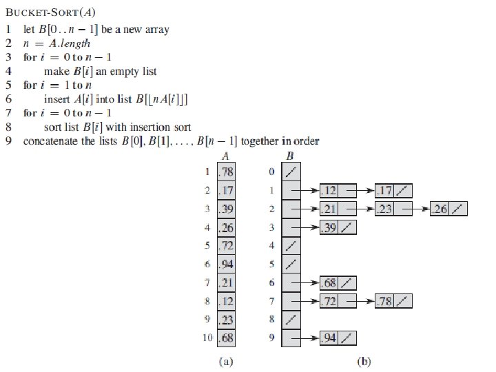
Bucket-Sort Let be S be a sequence of n (key, element) entries with keys in the range [0, N - 1] Bucket-sort uses the keys as indices into an auxiliary array B of sequences (buckets) Phase 1: Empty sequence S by moving each entry (k, o) into its bucket B[k] Phase 2: For i = 0, …, N - 1, move the entries of bucket B[i] to the end of sequence S Analysis: n n Phase 1 takes O(n) time Phase 2 takes O(n + N) time Bucket-sort takes O(n + N) time Goodrich, Tamassia Algorithm bucket. Sort(S, N) Input sequence S of (key, element) items with keys in the range [0, N - 1] Output sequence S sorted by increasing keys B array of N empty sequences while S. is. Empty() f S. first() (k, o) S. remove(f) B[k]. insert. Last((k, o)) for i 0 to N - 1 while B[i]. is. Empty() f B[i]. first() (k, o) B[i]. remove(f) S. insert. Last((k, o)) 57

Example Key range [0, 9] 7, d 1, c 3, a 7, g 3, b 7, e Phase 1 1, c B 3, a 0 1 1, c Goodrich, Tamassia 2 3 3, a 3, b 4 5 6 3, b 7 7, d 8 9 7, g 7, e Phase 2 7, d 7, g 7, e 58

Properties and Extensions Key-type Property n n The keys are used as indices into an array and cannot be arbitrary objects No external comparator Stable Sort Property n The relative order of any two items with the same key is preserved after the execution of the algorithm Goodrich, Tamassia Extensions n Integer keys in the range [a, b] w Put entry (k, o) into bucket B[k - a] n String keys from a set D of possible strings, where D has constant size (e. g. , names of the 50 U. S. states) w Sort D and compute the rank r(k) of each string k of D in the sorted sequence w Put entry (k, o) into bucket B[r(k)] 60

Radix-Sort in [G] Goodrich, Tamassia 61

Lexicographic Order A d-tuple is a sequence of d keys (k 1, k 2, …, kd), where key ki is said to be the i-th dimension of the tuple Example: n The Cartesian coordinates of a point in space are a 3 -tuple The lexicographic order of two d-tuples is recursively defined as follows (x 1, x 2, …, xd) < (y 1, y 2, …, yd) x 1 = y 1 (x 2, …, xd) < (y 2, …, yd) I. e. , the tuples are compared by the first dimension, then by the second dimension, etc. x 1 < y 1 Goodrich, Tamassia 62

Lexicographic-Sort Let Ci be the comparator that compares two tuples by their i-th dimension Let stable. Sort(S, C) be a stable sorting algorithm that uses comparator C Lexicographic-sorts a sequence of d-tuples in lexicographic order by executing d times algorithm stable. Sort, one per dimension Lexicographic-sort runs in O(d. T(n)) time, where T(n) is the running time of stable. Sort Goodrich, Tamassia Algorithm lexicographic. Sort(S) Input sequence S of d-tuples Output sequence S sorted in lexicographic order for i d downto 1 stable. Sort(S, Ci) Example: (7, 4, 6) (5, 1, 5) (2, 4, 6) (2, 1, 4) (3, 2, 4) (5, 1, 5) (7, 4, 6) (2, 1, 4) (5, 1, 5) (3, 2, 4) (7, 4, 6) (2, 1, 4) (2, 4, 6) (3, 2, 4) (5, 1, 5) (7, 4, 6) 63

Radix-Sort Radix-sort is a specialization of lexicographic-sort that uses bucket-sort as the stable sorting algorithm in each dimension Radix-sort is applicable to tuples where the keys in each dimension i are integers in the range [0, N - 1] Radix-sort runs in time O(d( n + N)) Goodrich, Tamassia Algorithm radix. Sort(S, N) Input sequence S of d-tuples such that (0, …, 0) (x 1, …, xd) and (x 1, …, xd) (N - 1, …, N - 1) for each tuple (x 1, …, xd) in S Output sequence S sorted in lexicographic order for i d downto 1 bucket. Sort(S, N) 64

Radix-Sort for Binary Numbers Consider a sequence of n bbit integers x = xb - 1 … x 1 x 0 We represent each element as a b-tuple of integers in the range [0, 1] and apply radix-sort with N = 2 This application of the radix -sort algorithm runs in O(bn) time For example, we can sort a sequence of 32 -bit integers in linear time Goodrich, Tamassia Algorithm binary. Radix. Sort(S) Input sequence S of b-bit integers Output sequence S sorted replace each element x of S with the item (0, x) for i 0 to b - 1 replace the key k of each item (k, x) of S with bit xi of x bucket. Sort(S, 2) 65

Example Sorting a sequence of 4 -bit integers Sorted 1001 0010 1001 0001 0010 1101 1001 0010 1001 0001 1101 0010 1101 1110 0001 1110 Goodrich, Tamassia 66

Selection in [G] Goodrich, Tamassia 67

The Selection Problem Given an integer k and n elements x 1, x 2, …, xn, taken from a total order, find the k-th smallest element in this set. Of course, we can sort the set in O(n log n) time and then index the k-th element. k=3 7 4 9 6 2 2 4 6 7 9 Can we solve the selection problem faster? Goodrich, Tamassia 68

Quick-Select Quick-select is a randomized selection algorithm based on the prune-and-search paradigm: n Prune: pick a random element x (called pivot) and partition S into w L elements less than x w E elements equal x w G elements greater than x Search: depending on k, either answer is in E, or we need to recurse in either L or G Goodrich, Tamassia x L k < |L| E G k > |L|+|E| k’ = k - |L| - |E| |L| < k < |L|+|E| (done) 69

Partition We partition an input sequence as in the quick-sort algorithm: n n We remove, in turn, each element y from S and We insert y into L, E or G, depending on the result of the comparison with the pivot x Each insertion and removal is at the beginning or at the end of a sequence, and hence takes O(1) time Thus, the partition step of quick-select takes O(n) time Goodrich, Tamassia Algorithm partition(S, p) Input sequence S, position p of pivot Output subsequences L, E, G of the elements of S less than, equal to, or greater than the pivot, resp. L, E, G empty sequences x S. remove(p) while S. is. Empty() y S. remove(S. first()) if y < x L. insert. Last(y) else if y = x E. insert. Last(y) else { y > x } G. insert. Last(y) return L, E, G 70

Quick-Select Visualization An execution of quick-select can be visualized by a recursion path n Each node represents a recursive call of quick-select, and stores k and the remaining sequence k=5, S=(7 4 9 3 2 6 5 1 8) k=2, S=(7 4 9 6 5 8) k=2, S=(7 4 6 5) k=1, S=(7 6 5) 5 Goodrich, Tamassia 71

Expected Running Time Consider a recursive call of quick-select on a sequence of size s n n Good call: the sizes of L and G are each less than 3 s/4 Bad call: one of L and G has size greater than 3 s/4 7 2 9 43 7 6 19 7 1 1 2 4 3 1 1 7294376 Good call Bad call A call is good with probability 1/2 n 1/2 of the possible pivots cause good calls: 1 2 3 4 5 6 7 8 9 10 11 12 13 14 15 16 Bad pivots Goodrich, Tamassia Good pivots Bad pivots 72

Deterministic Selection We can do selection in O(n) worst-case time. Main idea: recursively use the selection algorithm itself to find a good pivot for quick-select: n Divide S into n/5 sets of 5 each n Find a median in each set n Recursively find the median of the “baby” medians. Min size for L 1 1 1 2 3 4 2 3 4 2 3 4 5 5 5 Goodrich, Tamassia Min size for G 73

Reading • [G] Chapter 12: Sorting and Selection • [C] Chapter 8: Sorting in Linear Time • Repeated material • • [C] Chapter 9: Medians and Order Statistics [L] Section 7. 1: Sorting by Counting All about Trees is not required <yet> All about Graphs is not required <yet> 74

For Murtaja • x←x+y // x holds x + y, y holds y • y←x−y // x holds x + y, y holds x • x←x−y // x holds y, and y holds x • The same trick is applicable to any binary data by (XOR) operation: • Start: x=0100 y=1010 • x ← x XOR y x=1110 y=1010 • y ← x XOR y x=1110 y=0100 • x ← x XOR y x=1010 y=0100 75