SORTING 1 Sorting Sorting means arranging the elements

![Bubble Sort • Technique: • In Pass 1, A[0] and A[1] are compared, then Bubble Sort • Technique: • In Pass 1, A[0] and A[1] are compared, then](https://slidetodoc.com/presentation_image_h2/89052f0ede26aa7f383bd663b49295f2/image-15.jpg)

- Slides: 37

SORTING 1

Sorting • Sorting means arranging the elements of an array so that they are placed in some relevant order which may be either ascending or descending. • That is, if A is an array, then the elements of A are arranged in a sorted order (ascending order) in such a way that A[0] < A[1] < A[2] < … < A[N]. • The practical considerations for different sorting techniques would be: • Number of sort key comparisons that will be performed. • Number of times the records in the list will be moved. • Best, average and worst case performance. • Stability of the sorting algorithm where stability means that equivalent elements or records retain their relative positions even after sorting is done.

Sorting • Various sorting techniques are: • Insertion sort • Selection sort • Bubble sort • Merge sort • Quick sort • Radix sort • Bucket sort • Shell sort • Address calculation sort • Tree sort • Heap sort

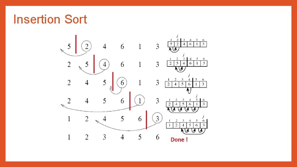
Insertion Sort • In insertion sort, the sorted array is built one at a time. • The main idea behind insertion sort is that it inserts each item into its proper place in the final list. • To save memory, most implementation of the insertion sort algorithm work by moving the current data element past the already sorted values and repeatedly interchanging it with the preceding value until it is in its correct place.

Insertion Sort • Technique: • The array of values to be sorted is divided into two sets. One that stores sorted values and another that contains unsorted values. • The sorting algorithm will proceed until there are elements in the unsorted set. • Suppose there are n elements in the array. Initially, the element with index 0 (assuming LB = 0) is in the sorted set. Rest of the elements are in the unsorted set. • The first element of the unsorted partition has array index 1 (if LB = 0) • During each iteration of the algorithm, the first element in the unsorted set is picked up and inserted into the correct position in the sorted set.

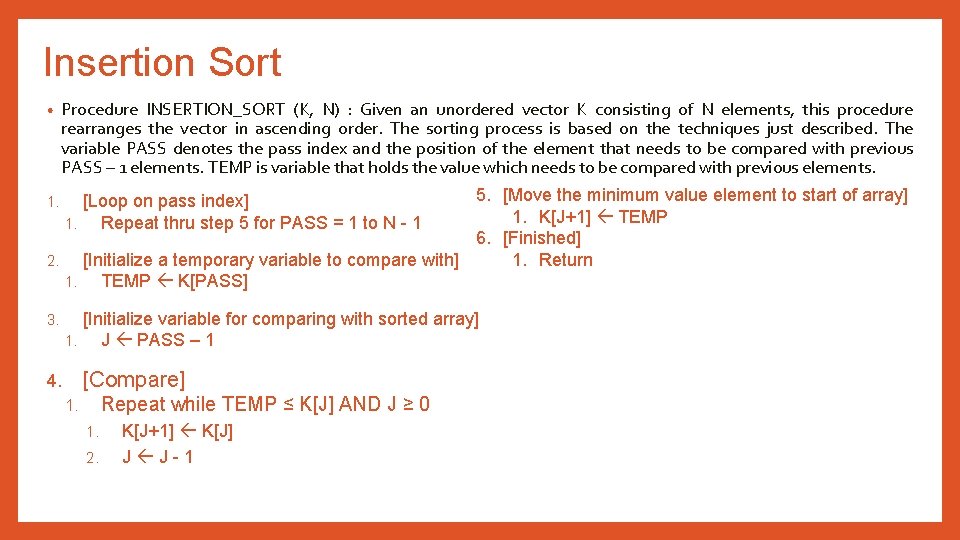
Insertion Sort • Procedure INSERTION_SORT (K, N) : Given an unordered vector K consisting of N elements, this procedure rearranges the vector in ascending order. The sorting process is based on the techniques just described. The variable PASS denotes the pass index and the position of the element that needs to be compared with previous PASS – 1 elements. TEMP is variable that holds the value which needs to be compared with previous elements. 5. [Move the minimum value element to start of array] 1. K[J+1] TEMP 6. [Finished] 1. Return 2. [Initialize a temporary variable to compare with] 1. TEMP K[PASS] 1. [Loop on pass index] 1. Repeat thru step 5 for PASS = 1 to N - 1 3. [Initialize variable for comparing with sorted array] 1. J PASS – 1 [Compare] 4. Repeat while TEMP ≤ K[J] AND J ≥ 0 1. 1. 2. K[J+1] K[J] J J-1

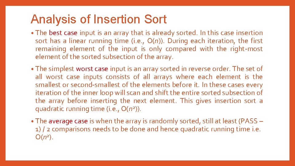
Analysis of Insertion Sort • The best case input is an array that is already sorted. In this case insertion sort has a linear running time (i. e. , O(n)). During each iteration, the first remaining element of the input is only compared with the right-most element of the sorted subsection of the array. • The simplest worst case input is an array sorted in reverse order. The set of all worst case inputs consists of all arrays where each element is the smallest or second-smallest of the elements before it. In these cases every iteration of the inner loop will scan and shift the entire sorted subsection of the array before inserting the next element. This gives insertion sort a quadratic running time (i. e. , O(n 2)). • The average case is when the array is randomly sorted, still at least (PASS – 1) / 2 comparisons needs to be done and hence quadratic running time i. e. O(n 2).

Insertion Sort

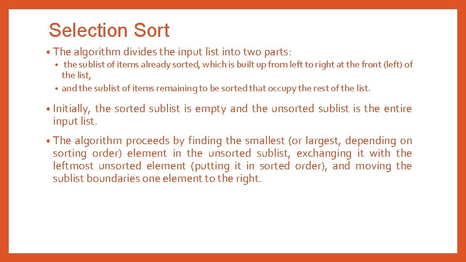
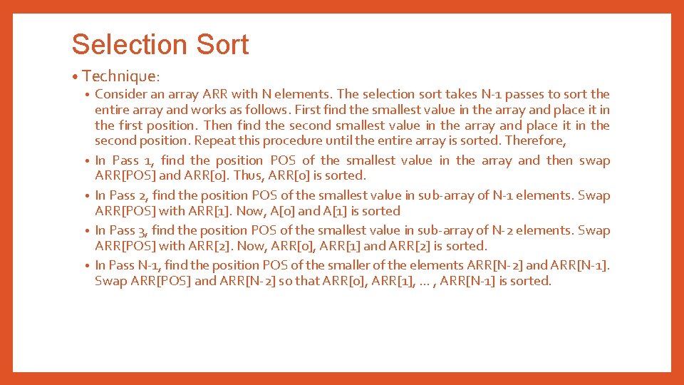
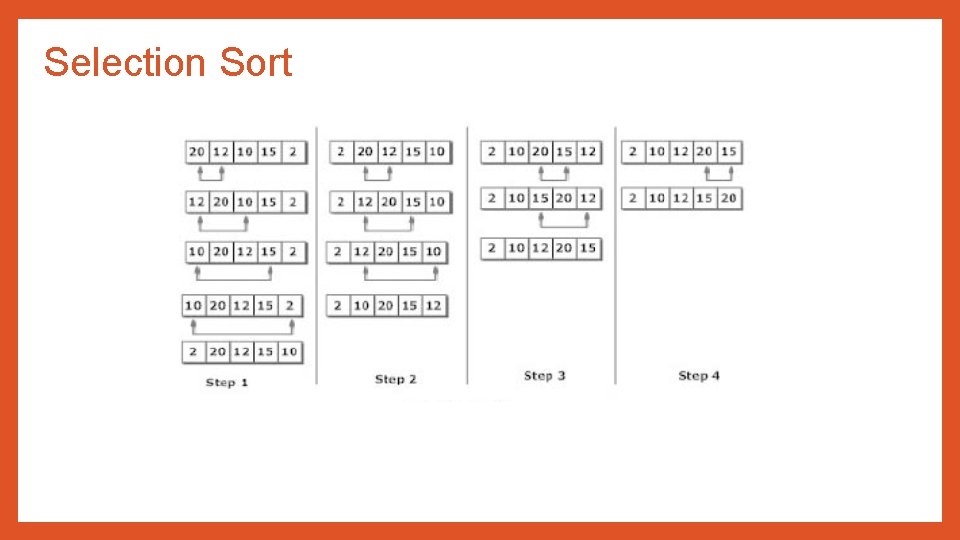
Selection Sort • The algorithm divides the input list into two parts: • the sublist of items already sorted, which is built up from left to right at the front (left) of the list, • and the sublist of items remaining to be sorted that occupy the rest of the list. • Initially, the sorted sublist is empty and the unsorted sublist is the entire input list. • The algorithm proceeds by finding the smallest (or largest, depending on sorting order) element in the unsorted sublist, exchanging it with the leftmost unsorted element (putting it in sorted order), and moving the sublist boundaries one element to the right.

Selection Sort • Technique: • Consider an array ARR with N elements. The selection sort takes N-1 passes to sort the entire array and works as follows. First find the smallest value in the array and place it in the first position. Then find the second smallest value in the array and place it in the second position. Repeat this procedure until the entire array is sorted. Therefore, • In Pass 1, find the position POS of the smallest value in the array and then swap ARR[POS] and ARR[0]. Thus, ARR[0] is sorted. • In Pass 2, find the position POS of the smallest value in sub-array of N-1 elements. Swap ARR[POS] with ARR[1]. Now, A[0] and A[1] is sorted • In Pass 3, find the position POS of the smallest value in sub-array of N-2 elements. Swap ARR[POS] with ARR[2]. Now, ARR[0], ARR[1] and ARR[2] is sorted. • In Pass N-1, find the position POS of the smaller of the elements ARR[N-2] and ARR[N-1]. Swap ARR[POS] and ARR[N-2] so that ARR[0], ARR[1], … , ARR[N-1] is sorted.

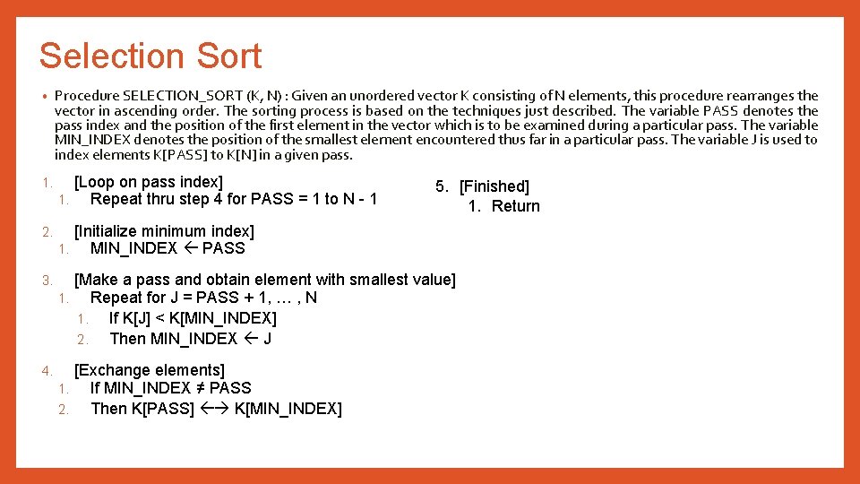
Selection Sort • Procedure SELECTION_SORT (K, N) : Given an unordered vector K consisting of N elements, this procedure rearranges the vector in ascending order. The sorting process is based on the techniques just described. The variable PASS denotes the pass index and the position of the first element in the vector which is to be examined during a particular pass. The variable MIN_INDEX denotes the position of the smallest element encountered thus far in a particular pass. The variable J is used to index elements K[PASS] to K[N] in a given pass. 1. [Loop on pass index] 1. Repeat thru step 4 for PASS = 1 to N - 1 2. [Initialize minimum index] 1. MIN_INDEX PASS 3. [Make a pass and obtain element with smallest value] 1. Repeat for J = PASS + 1, … , N 1. If K[J] < K[MIN_INDEX] 2. Then MIN_INDEX J 4. [Exchange elements] 1. If MIN_INDEX ≠ PASS 2. Then K[PASS] K[MIN_INDEX] 5. [Finished] 1. Return

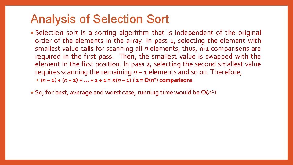
Analysis of Selection Sort • Selection sort is a sorting algorithm that is independent of the original order of the elements in the array. In pass 1, selecting the element with smallest value calls for scanning all n elements; thus, n-1 comparisons are required in the first pass. Then, the smallest value is swapped with the element in the first position. In pass 2, selecting the second smallest value requires scanning the remaining n − 1 elements and so on. Therefore, • • (n − 1) + (n − 2) +. . . + 2 + 1 = n(n − 1) / 2 = O(n 2) comparisons So, for best, average and worst case, running time would be O(n 2).

Selection Sort

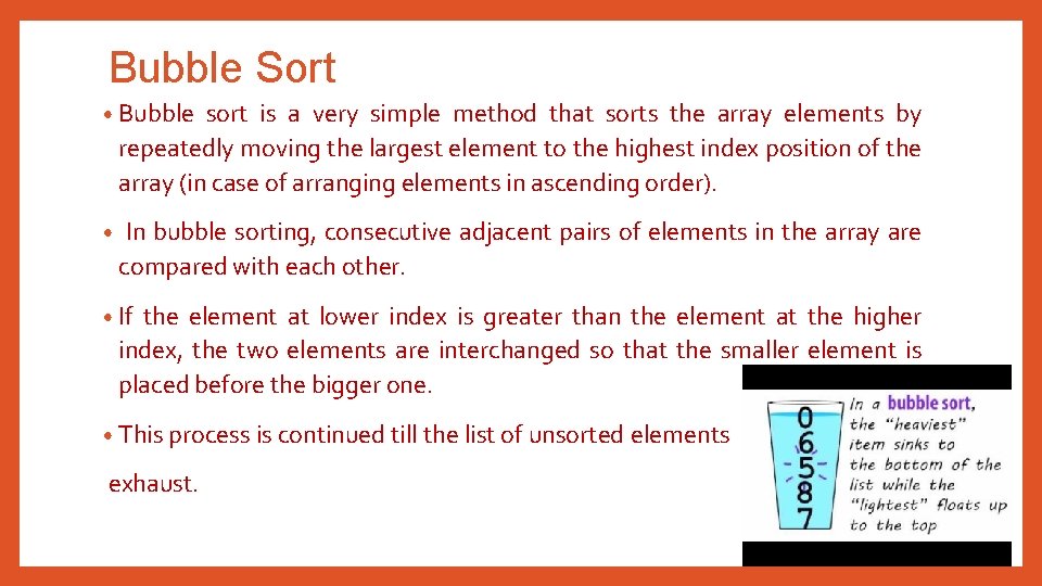
Bubble Sort • Bubble sort is a very simple method that sorts the array elements by repeatedly moving the largest element to the highest index position of the array (in case of arranging elements in ascending order). • In bubble sorting, consecutive adjacent pairs of elements in the array are compared with each other. • If the element at lower index is greater than the element at the higher index, the two elements are interchanged so that the smaller element is placed before the bigger one. • This process is continued till the list of unsorted elements exhaust.
![Bubble Sort Technique In Pass 1 A0 and A1 are compared then Bubble Sort • Technique: • In Pass 1, A[0] and A[1] are compared, then](https://slidetodoc.com/presentation_image_h2/89052f0ede26aa7f383bd663b49295f2/image-15.jpg)
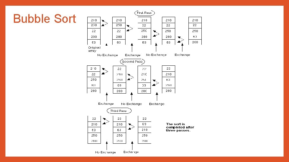
Bubble Sort • Technique: • In Pass 1, A[0] and A[1] are compared, then A[1] is compared with A[2], A[2] is compared with A[3] and so on. Finally, A[N-2] is compared with A[N-1]. Pass 1 involves N-1 comparisons and places the biggest element at the highest index of the array. • In Pass 2, A[0] and A[1] are compared. then A[1] is compared with A[2], A[2] is compared with A[3] and so on. Finally, A[N-3] is compared with A[N-2]. Pass 2 involves N-2 comparisons and places the second biggest element at the second highest index of the array. • In Pass 3, A[0] and A[1] are compared. then A[1] is compared with A[2], A[2] is compared with A[3] and so on. Finally, A[N-4] is compared with A[N-3]. Pass 3 involves N-3 comparisons and places the third biggest element at the third highest index of the array. • In Pass n-1, A[0] and A[1] are compared so that A[0] < A[1]. After this step, all the elements of the array are arranged in ascending order.

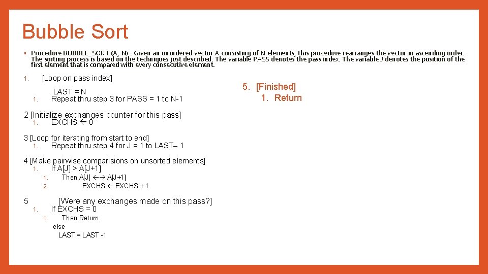
Bubble Sort • Procedure BUBBLE_SORT (A, N) : Given an unordered vector A consisting of N elements, this procedure rearranges the vector in ascending order. The sorting process is based on the techniques just described. The variable PASS denotes the pass index. The variable J denotes the position of the first element that is compared with every consecutive element. [Loop on pass index] 1. LAST = N Repeat thru step 3 for PASS = 1 to N-1 1. 2 [Initialize exchanges counter for this pass] EXCHS 0 1. 3 [Loop for iterating from start to end] 1. Repeat thru step 4 for J = 1 to LAST– 1 4 [Make pairwise comparisions on unsorted elements] 1. If A[J] > A[J+1] 1. 2. 5 Then A[J] A[J+1] EXCHS + 1 [Were any exchanges made on this pass? ] If EXCHS = 0 1. 1. Then Return else LAST = LAST -1 5. [Finished] 1. Return

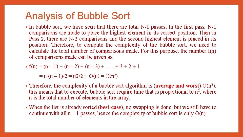
Analysis of Bubble Sort • In bubble sort, we have seen that there are total N-1 passes. In the first pass, N-1 comparisons are made to place the highest element in its correct position. Then in Pass 2, there are N-2 comparisons and the second highest element is placed in its position. Therefore, to compute the complexity of the bubble sort, we need to calculate the total number of comparisons made. For this purpose, the number f(n) of comparisons made can be given as, • f(n) = (n – 1) + (n – 2) + (n – 3) + …. . + 3 + 2 + 1 = n (n – 1)/2 = n 2/2 + O(n) = O(n 2) • Therefore, the complexity of a bubble sort algorithm is (average and worst) O(n 2), this means that to execute, bubble sort require time that is proportional to n 2, where n is the total number of elements in the array. • When the list is already sorted (best-case), no swapping is done, but we still have to continue with all n – 1 passes, hence the complexity of bubble sort is only O(n).

Bubble Sort

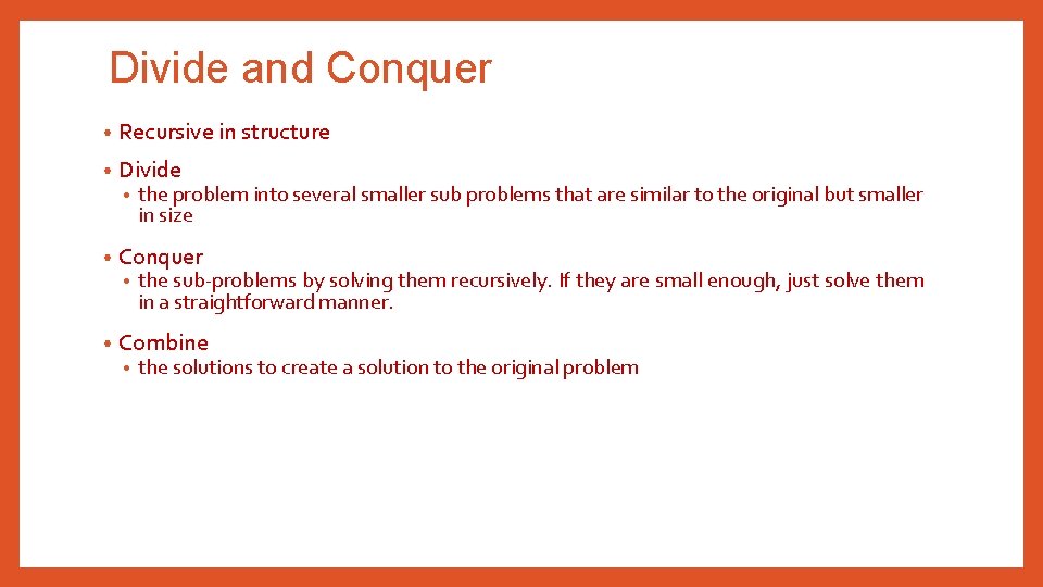
Divide and Conquer • Recursive in structure • Divide • • Conquer • • the problem into several smaller sub problems that are similar to the original but smaller in size the sub-problems by solving them recursively. If they are small enough, just solve them in a straightforward manner. Combine • the solutions to create a solution to the original problem

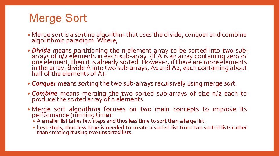
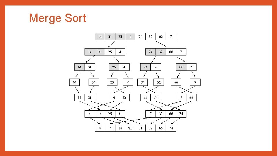
Merge Sort • Merge sort is a sorting algorithm that uses the divide, conquer and combine algorithmic paradigm. Where, • Divide means partitioning the n-element array to be sorted into two subarrays of n/2 elements in each sub-array. (If A is an array containing zero or one element, then it is already sorted. However, if there are more elements in the array, divide A into two sub-arrays, A 1 and A 2, each containing about half of the elements of A). • Conquer means sorting the two sub-arrays recursively using merge sort. • Combine means merging the two sorted sub-arrays of size n/2 each to produce the sorted array of n elements. • Merge sort algorithms focuses on two main concepts to improve its performance (running time): • • A smaller list takes few steps and thus less time to sort than a large list. Less steps, thus less time is needed to create a sorted list from two sorted lists rather than creating it using two unsorted lists.

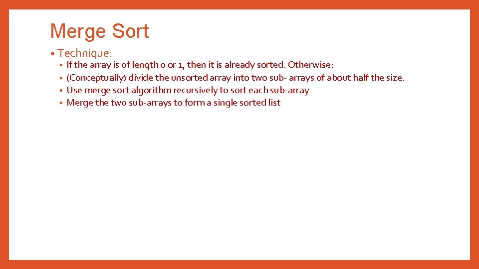
Merge Sort • Technique: • If the array is of length 0 or 1, then it is already sorted. Otherwise: • (Conceptually) divide the unsorted array into two sub- arrays of about half the size. • Use merge sort algorithm recursively to sort each sub-array • Merge the two sub-arrays to form a single sorted list

Merge Sort

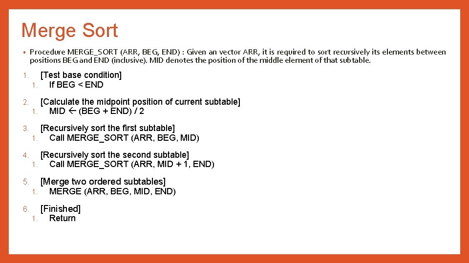
Merge Sort • Procedure MERGE_SORT (ARR, BEG, END) : Given an vector ARR, it is required to sort recursively its elements between positions BEG and END (inclusive). MID denotes the position of the middle element of that subtable. 1. [Test base condition] 1. If BEG < END 2. [Calculate the midpoint position of current subtable] 1. MID (BEG + END) / 2 3. [Recursively sort the first subtable] 1. Call MERGE_SORT (ARR, BEG, MID) 4. [Recursively sort the second subtable] 1. Call MERGE_SORT (ARR, MID + 1, END) [Merge two ordered subtables] 5. 1. MERGE (ARR, BEG, MID, END) [Finished] 6. 1. Return

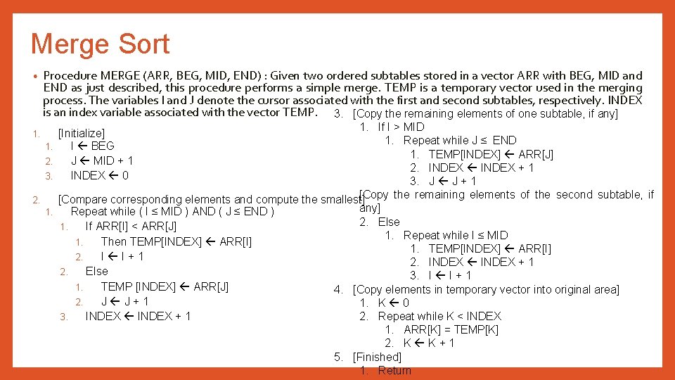
Merge Sort • Procedure MERGE (ARR, BEG, MID, END) : Given two ordered subtables stored in a vector ARR with BEG, MID and END as just described, this procedure performs a simple merge. TEMP is a temporary vector used in the merging process. The variables I and J denote the cursor associated with the first and second subtables, respectively. INDEX is an index variable associated with the vector TEMP. 3. [Copy the remaining elements of one subtable, if any] 1. If I > MID 1. Repeat while J ≤ END 1. TEMP[INDEX] ARR[J] 2. INDEX + 1 3. J J + 1 [Copy the remaining elements of the second subtable, if 2. [Compare corresponding elements and compute the smallest] any] 1. Repeat while ( I ≤ MID ) AND ( J ≤ END ) 2. Else 1. If ARR[I] < ARR[J] 1. Repeat while I ≤ MID 1. Then TEMP[INDEX] ARR[I] 1. TEMP[INDEX] ARR[I] 2. I I+1 2. INDEX + 1 2. Else 3. I I + 1 1. TEMP [INDEX] ARR[J] 4. [Copy elements in temporary vector into original area] 2. J J+1 1. K 0 2. Repeat while K < INDEX 3. INDEX + 1 1. ARR[K] = TEMP[K] 2. K K + 1 5. [Finished] 1. Return 1. [Initialize] 1. I BEG 2. J MID + 1 3. INDEX 0

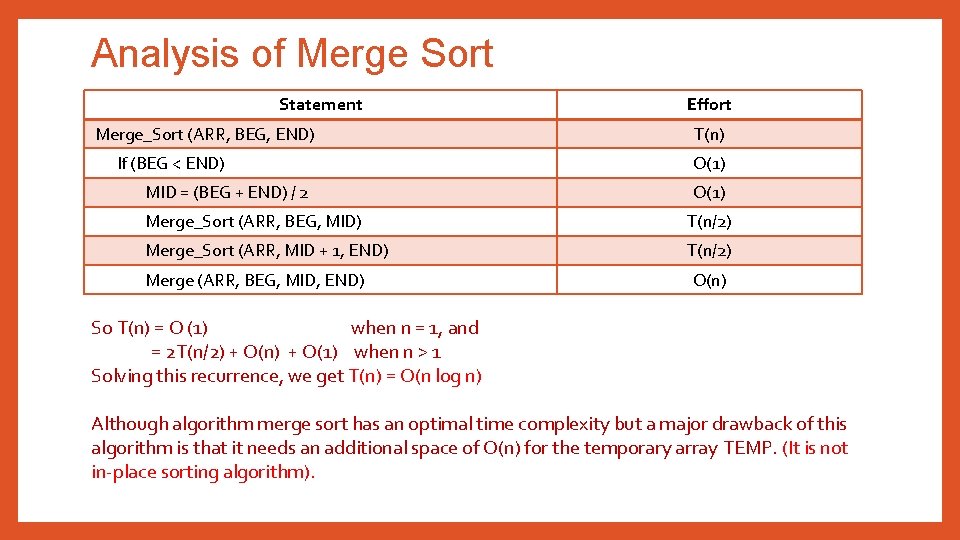
Analysis of Merge Sort Statement Merge_Sort (ARR, BEG, END) If (BEG < END) MID = (BEG + END) / 2 Effort T(n) O(1) Merge_Sort (ARR, BEG, MID) T(n/2) Merge_Sort (ARR, MID + 1, END) T(n/2) Merge (ARR, BEG, MID, END) O(n) So T(n) = O (1) when n = 1, and = 2 T(n/2) + O(n) + O(1) when n > 1 Solving this recurrence, we get T(n) = O(n log n) Although algorithm merge sort has an optimal time complexity but a major drawback of this algorithm is that it needs an additional space of O(n) for the temporary array TEMP. (It is not in-place sorting algorithm).

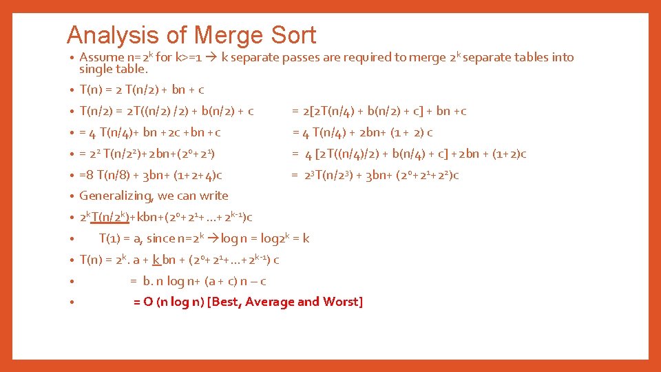
Analysis of Merge Sort • Assume n=2 k for k>=1 k separate passes are required to merge 2 k separate tables into single table. • T(n) = 2 T(n/2) + bn + c • T(n/2) = 2 T((n/2) + b(n/2) + c = 2[2 T(n/4) + b(n/2) + c] + bn +c • = 4 T(n/4)+ bn +2 c +bn +c = 4 T(n/4) + 2 bn+ (1 + 2) c • = 22 T(n/22)+2 bn+(20+21) = 4 [2 T((n/4)/2) + b(n/4) + c] +2 bn + (1+2)c • =8 T(n/8) + 3 bn+ (1+2+4)c = 23 T(n/23) + 3 bn+ (20+21+22)c • Generalizing, we can write • 2 k. T(n/2 k)+kbn+(20+21+. . . +2 k-1)c • • T(1) = a, since n=2 k log n = log 2 k = k T(n) = 2 k. a + k bn + (20+21+. . . +2 k-1) c • = b. n log n+ (a + c) n – c • = O (n log n) [Best, Average and Worst]

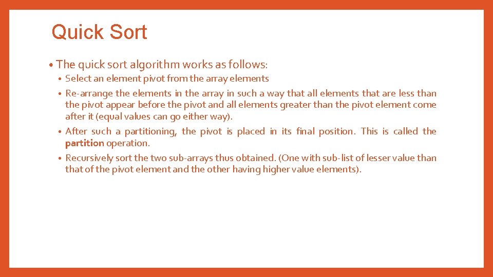
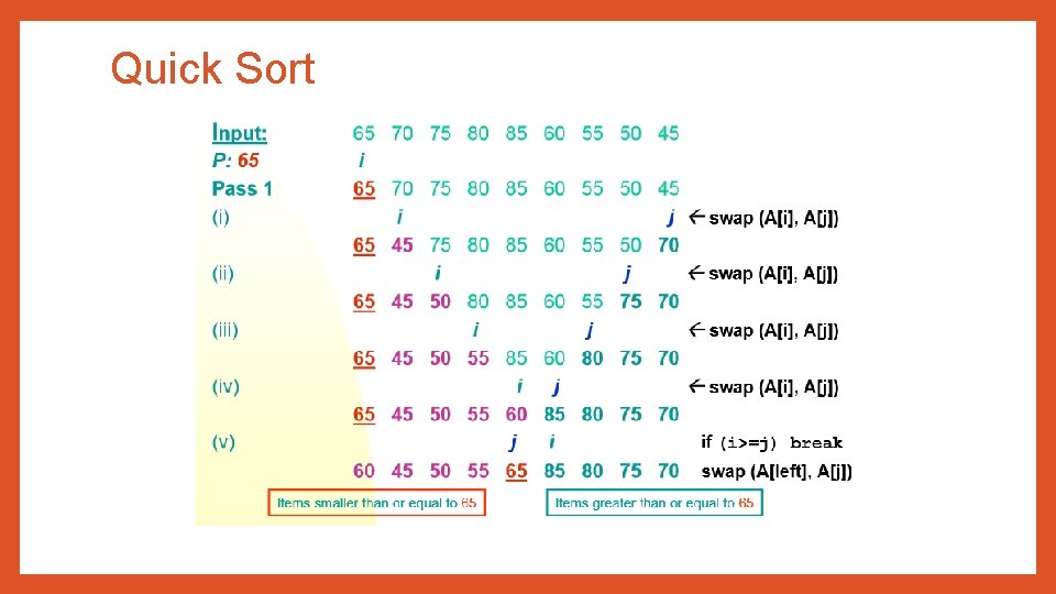
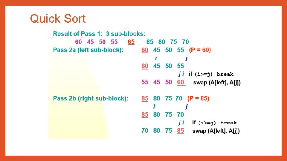
Quick Sort • The quick sort algorithm works as follows: • Select an element pivot from the array elements • Re-arrange the elements in the array in such a way that all elements that are less than the pivot appear before the pivot and all elements greater than the pivot element come after it (equal values can go either way). • After such a partitioning, the pivot is placed in its final position. This is called the partition operation. • Recursively sort the two sub-arrays thus obtained. (One with sub-list of lesser value than that of the pivot element and the other having higher value elements).

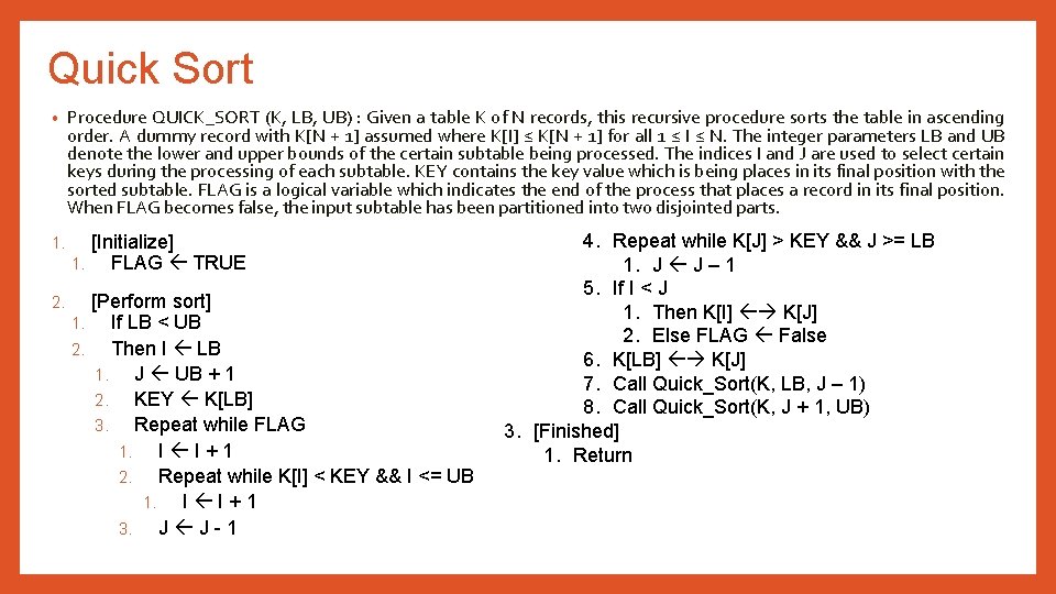
Quick Sort • Procedure QUICK_SORT (K, LB, UB) : Given a table K of N records, this recursive procedure sorts the table in ascending order. A dummy record with K[N + 1] assumed where K[I] ≤ K[N + 1] for all 1 ≤ I ≤ N. The integer parameters LB and UB denote the lower and upper bounds of the certain subtable being processed. The indices I and J are used to select certain keys during the processing of each subtable. KEY contains the key value which is being places in its final position with the sorted subtable. FLAG is a logical variable which indicates the end of the process that places a record in its final position. When FLAG becomes false, the input subtable has been partitioned into two disjointed parts. 1. [Initialize] 1. FLAG TRUE 2. [Perform sort] 1. If LB < UB 2. Then I LB 1. J UB + 1 2. KEY K[LB] 3. Repeat while FLAG 1. I I+1 2. Repeat while K[I] < KEY && I <= UB 1. I I+1 3. J J-1 4. Repeat while K[J] > KEY && J >= LB 1. J J – 1 5. If I < J 1. Then K[I] K[J] 2. Else FLAG False 6. K[LB] K[J] 7. Call Quick_Sort(K, LB, J – 1) 8. Call Quick_Sort(K, J + 1, UB) 3. [Finished] 1. Return

Quick Sort

Quick Sort

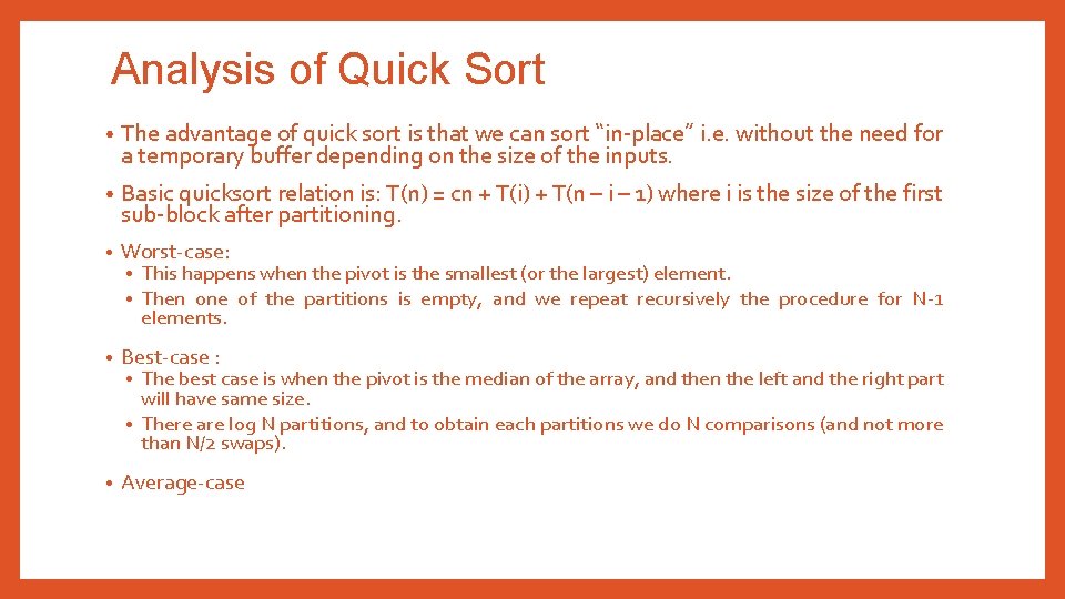
Analysis of Quick Sort • The advantage of quick sort is that we can sort “in-place” i. e. without the need for a temporary buffer depending on the size of the inputs. • Basic quicksort relation is: T(n) = cn + T(i) + T(n – i – 1) where i is the size of the first sub-block after partitioning. • Worst-case: • Best-case : • Average-case • • This happens when the pivot is the smallest (or the largest) element. Then one of the partitions is empty, and we repeat recursively the procedure for N-1 elements. The best case is when the pivot is the median of the array, and then the left and the right part will have same size. • There are log N partitions, and to obtain each partitions we do N comparisons (and not more than N/2 swaps). •

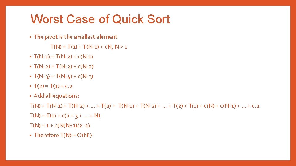
Worst Case of Quick Sort • The pivot is the smallest element T(N) = T(1) + T(N-1) + c. N, N > 1 • T(N-1) = T(N-2) + c(N-1) • T(N-2) = T(N-3) + c(N-2) • T(N-3) = T(N-4) + c(N-3) • T(2) = T(1) + c. 2 • Add all equations: T(N) + T(N-1) + T(N-2) + … + T(2) = T(N-1) + T(N-2) + … + T(2) + T(1) + c(N-1) + … + c. 2 T(N) = T(1) + c(2 + 3 + … + N) T(N) = 1 + c(N(N+1)/2 -1) • Therefore T(N) = O(N 2)

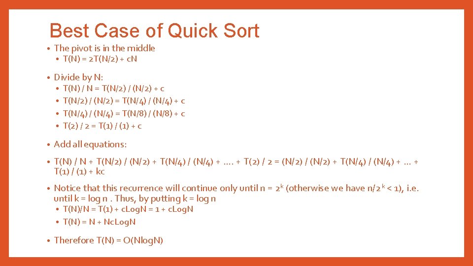
Best Case of Quick Sort • The pivot is in the middle • • T(N) = 2 T(N/2) + c. N Divide by N: T(N) / N = T(N/2) / (N/2) + c • T(N/2) / (N/2) = T(N/4) / (N/4) + c • T(N/4) / (N/4) = T(N/8) / (N/8) + c • T(2) / 2 = T(1) / (1) + c • • Add all equations: • T(N) / N + T(N/2) / (N/2) + T(N/4) / (N/4) + …. + T(2) / 2 = (N/2) / (N/2) + T(N/4) / (N/4) + … + T(1) / (1) + kc • Notice that this recurrence will continue only until n = 2 k (otherwise we have n/2 k < 1), i. e. until k = log n. Thus, by putting k = log n T(N)/N = T(1) + c. Log. N = 1 + c. Log. N • T(N) = N + Nc. Log. N • • Therefore T(N) = O(Nlog. N)

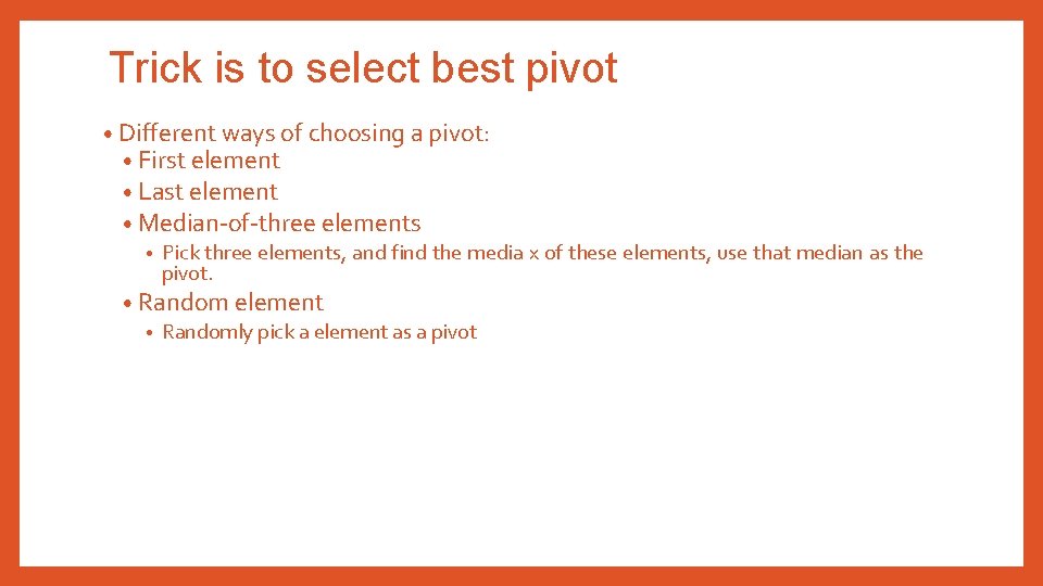
Trick is to select best pivot • Different ways of choosing a pivot: • First element • Last element • Median-of-three elements • Pick three elements, and find the media x of these elements, use that median as the pivot. • Random element • Randomly pick a element as a pivot

Radix Sort • Radix sort is one of the linear sorting algorithms for integers. • Radix sort is a non-comparative integer sorting algorithm that sorts data with integer keys by grouping keys by the individual digits which share the same significant position and value. • It functions by sorting the input numbers on each digit, for each of the digits in the numbers. • However, the process adopted by this sort method is somewhat counterintuitive, in the sense that the numbers are sorted on the leastsignificant digit first, followed by the second-least significant digit and so on till the most significant digit.

Radix Sort • Each key is first figuratively dropped into one level of buckets corresponding to the value of the rightmost digit. • Each bucket preserves the original order of the keys as the keys are dropped into the bucket. • There is a one-to-one correspondence between the buckets and the values that can be represented by the rightmost digit. Then, the process repeats with the next neighbouring more significant digit until there are no more digits to process. In other words: Take the least significant digit (or group of bits, both being examples of radices) of each key. • Group the keys based on that digit, but otherwise keep the original order of keys. (This is what makes the LSD radix sort a stable sort. ) • Repeat the grouping process with each more significant digit. •

THANK YOU!! ANY QUESTIONS? ? 37