Reporting your results From RCommander to the Results

How to reports results from RCommander Finding Means and Standard Deviations Independent Paired samples

Means and Standard Deviations mean sd n Conservative 72. 65714 13. 89714 35 Liberal

Independent samples t-test Two Sample t-test data: Moral by Pol_grp t = 2. 1246,

Independent samples t-test An independent samples t-test indicate that there was a significant difference

Paired Samples t-test Paired t-test data: After and Before t = 5. 4704, df

Independent samples t-test An paired samples t-test indicate that there was a significant difference

One-way between subjects ANOVA Df Sum Sq Mean Sq F value Pr(>F) Condition 2

One-way between subjects ANOVA The one-way ANOVA indicated that there was a significant effect

One-way repeated measures ANOVA Sum Sq Df Error SS den Df F value (Intercept)

One-way repeated measures ANOVA The repeated measures one-way ANOVA indicated that there was a

Factorial between subjects ANOVA Sum Sq Df F value Pr(>F) (Intercept) 459901 1 2541.

Factorial between subjects ANOVA A 3 x 2 ANOVA was conducted to examine whether

Two-way repeated measures ANOVA Sum Sq num Df Error SS den Df F value

Two-way repeated measures A 3 x 2 ANOVA was conducted to examine whether judgments

Correlation Pearson's product-moment correlation data: Inter and PVD t = 1. 2724, df =

Simple regression Coefficients: Estimate Std. Error t value Pr(>|t|) (Intercept) 63. 547 7. 931

Simple regression A simple regression indicated that interpersonal disgust did explain a significant amount

Multiple regression Coefficients: Estimate Std. Error t value Pr(>|t|) (Intercept) 87. 3278 9. 7917

Multiple regression A multiple regression analysis indicated that core, interpersonal, and death/body disgust sensitivity

Slides: 30

Download presentation

Reporting your results From RCommander to the Results section

How to reports results from RCommander Finding Means and Standard Deviations Independent Paired samples t-test One-way ANOVA (RM ANOVA) Factorial ANOVA (RM Factorial ANOVA) Correlation Regression

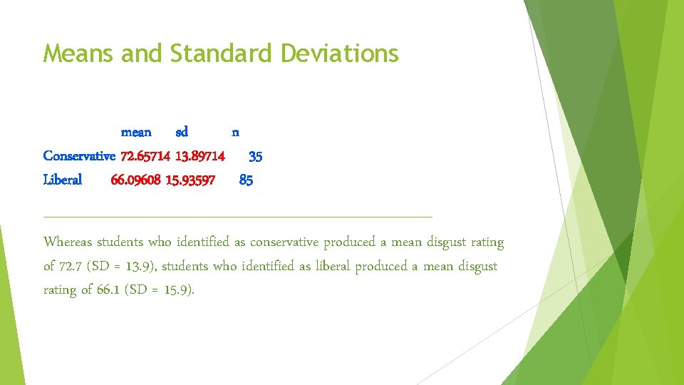
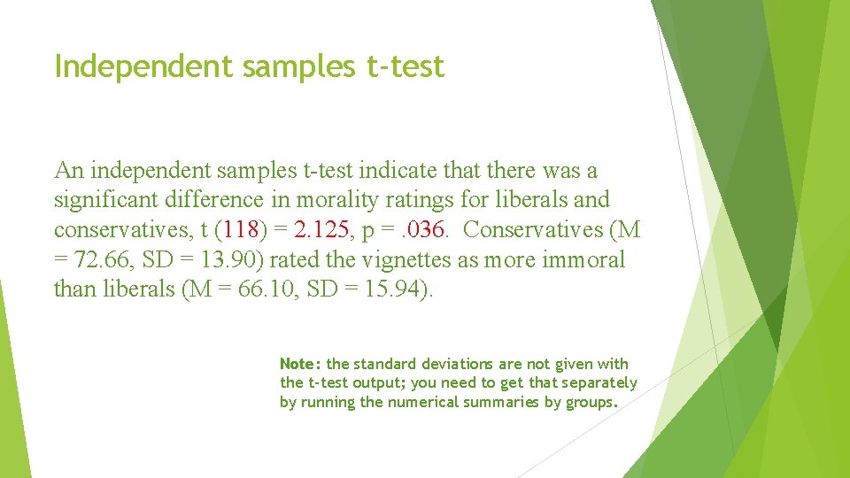
Means and Standard Deviations mean sd n Conservative 72. 65714 13. 89714 35 Liberal 66. 09608 15. 93597 85 ____________________ Whereas students who identified as conservative produced a mean disgust rating of 72. 7 (SD = 13. 9), students who identified as liberal produced a mean disgust rating of 66. 1 (SD = 15. 9).

How to reports results from RCommander Finding Means and Standard Deviations Independent Paired samples t-test One-way ANOVA (RM ANOVA) Factorial ANOVA (RM Factorial ANOVA) Correlation Regression

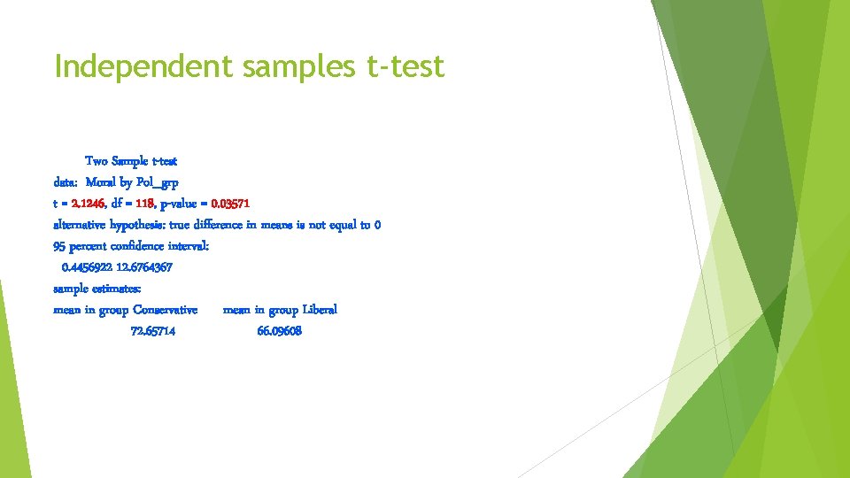
Independent samples t-test Two Sample t-test data: Moral by Pol_grp t = 2. 1246, df = 118, p-value = 0. 03571 alternative hypothesis: true difference in means is not equal to 0 95 percent confidence interval: 0. 4456922 12. 6764367 sample estimates: mean in group Conservative mean in group Liberal 72. 65714 66. 09608

Independent samples t-test An independent samples t-test indicate that there was a significant difference in morality ratings for liberals and conservatives, t (118) = 2. 125, p =. 036. Conservatives (M = 72. 66, SD = 13. 90) rated the vignettes as more immoral than liberals (M = 66. 10, SD = 15. 94). Note: the standard deviations are not given with the t-test output; you need to get that separately by running the numerical summaries by groups.

How to reports results from RCommander Finding Means and Standard Deviations Independent Paired samples t-test One-way ANOVA (RM ANOVA) Factorial ANOVA (RM Factorial ANOVA) Correlation Regression

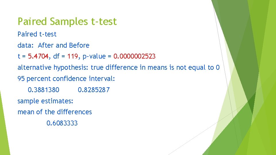
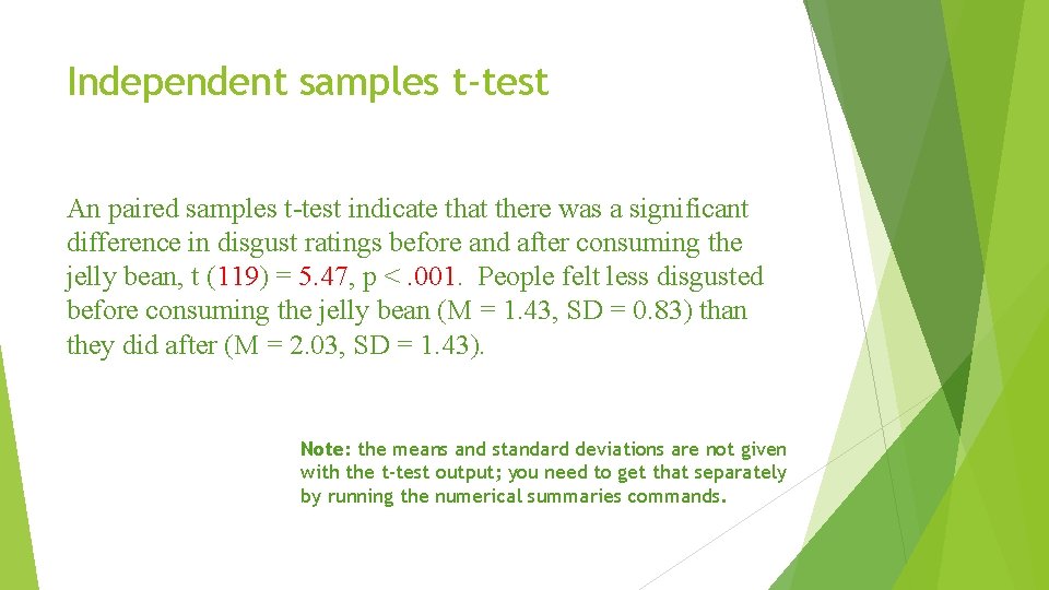
Paired Samples t-test Paired t-test data: After and Before t = 5. 4704, df = 119, p-value = 0. 0000002523 alternative hypothesis: true difference in means is not equal to 0 95 percent confidence interval: 0. 3881380 0. 8285287 sample estimates: mean of the differences 0. 6083333

Independent samples t-test An paired samples t-test indicate that there was a significant difference in disgust ratings before and after consuming the jelly bean, t (119) = 5. 47, p <. 001. People felt less disgusted before consuming the jelly bean (M = 1. 43, SD = 0. 83) than they did after (M = 2. 03, SD = 1. 43). Note: the means and standard deviations are not given with the t-test output; you need to get that separately by running the numerical summaries commands.

How to reports results from RCommander Finding Means and Standard Deviations Independent Paired samples t-test One-way ANOVA (RM ANOVA) Factorial ANOVA (RM Factorial ANOVA) Correlation Regression

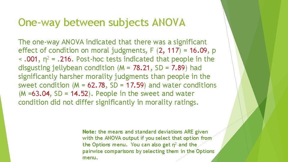
One-way between subjects ANOVA Df Sum Sq Mean Sq F value Pr(>F) Condition 2 6247 3123. 6 16. 09 6. 73 e-07 *** Residuals 117 22719 194. 2 part. eta sq. Condition 0. 2157 Linear Hypotheses: Estimate Std. Error t value Pr(>|t|) Sweet - Disgusting == 0 -15. 4333 3. 1159 -4. 953 <1 e-05 *** Water - Disgusting == 0 -15. 1750 3. 1159 -4. 870 <1 e-05 *** Water - Sweet == 0 3. 1159 0. 083 0. 996 0. 2583 --Signif. codes: 0 '***' 0. 001 '**' 0. 01 '*' 0. 05 '. ' 0. 1 ' ' 1

One-way between subjects ANOVA The one-way ANOVA indicated that there was a significant effect of condition on moral judgments, F (2, 117) = 16. 09, p <. 001, η 2 =. 216. Post-hoc tests indicated that people in the disgusting jellybean condition (M = 78. 21, SD = 7. 89) had significantly harsher morality judgments than people in the sweet condition (M = 62. 78, SD = 17. 59) and water conditions (M =63. 04, SD = 14. 52). People in the sweet and water condition did not differ significantly in morality ratings. Note: the means and standard deviations ARE given with the ANOVA output if you select that option from the Options menu. You can also get η 2 and the pairwise comparisons by selecting them in the Options menu.

How to reports results from RCommander Finding Means and Standard Deviations Independent Paired samples t-test One-way ANOVA (RM ANOVA) Factorial ANOVA (RM Factorial ANOVA) Correlation Regression

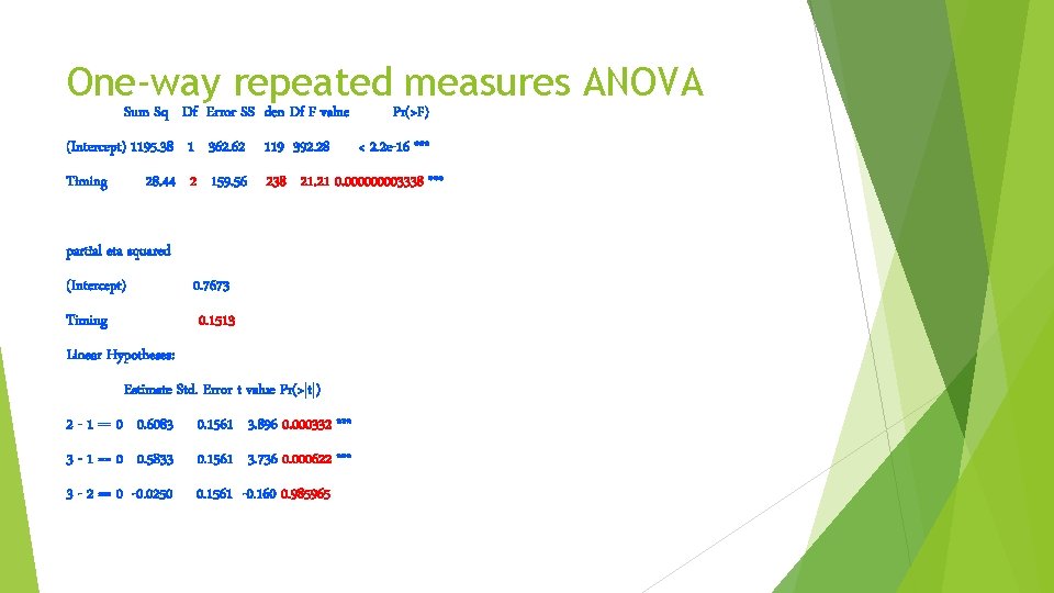
One-way repeated measures ANOVA Sum Sq Df Error SS den Df F value (Intercept) 1195. 38 1 362. 62 119 392. 28 Timing Pr(>F) < 2. 2 e-16 *** 28. 44 2 159. 56 238 21. 21 0. 00003338 *** partial eta squared (Intercept) 0. 7673 Timing 0. 1513 Linear Hypotheses: Estimate Std. Error t value Pr(>|t|) 2 - 1 == 0 0. 6083 0. 1561 3. 896 0. 000332 *** 3 - 1 == 0 0. 5833 0. 1561 3. 736 0. 000622 *** 3 - 2 == 0 -0. 0250 0. 1561 -0. 160 0. 985965

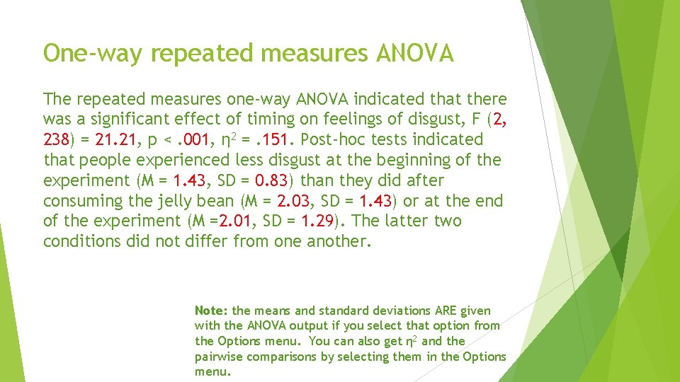
One-way repeated measures ANOVA The repeated measures one-way ANOVA indicated that there was a significant effect of timing on feelings of disgust, F (2, 238) = 21. 21, p <. 001, η 2 =. 151. Post-hoc tests indicated that people experienced less disgust at the beginning of the experiment (M = 1. 43, SD = 0. 83) than they did after consuming the jelly bean (M = 2. 03, SD = 1. 43) or at the end of the experiment (M =2. 01, SD = 1. 29). The latter two conditions did not differ from one another. Note: the means and standard deviations ARE given with the ANOVA output if you select that option from the Options menu. You can also get η 2 and the pairwise comparisons by selecting them in the Options menu.

How to reports results from RCommander Finding Means and Standard Deviations Independent Paired samples t-test One-way ANOVA (RM ANOVA) Factorial ANOVA (RM Factorial ANOVA) Correlation Regression

Factorial between subjects ANOVA Sum Sq Df F value Pr(>F) (Intercept) 459901 1 2541. 7059 < 2. 2 e-16 *** Condition 4542 2 12. 5496 0. 00001 *** Pol_grp 592 1 3. 2713 0. 07314. Condition: Pol_grp 1437 2 3. 9707 0. 02153 * Residuals 20627 114 part. eta sq. (Intercept) 0. 9442 Condition 0. 0093 Pol_grp 0. 0012 Condition: Pol_grp Residuals 0. 0029 0. 0423

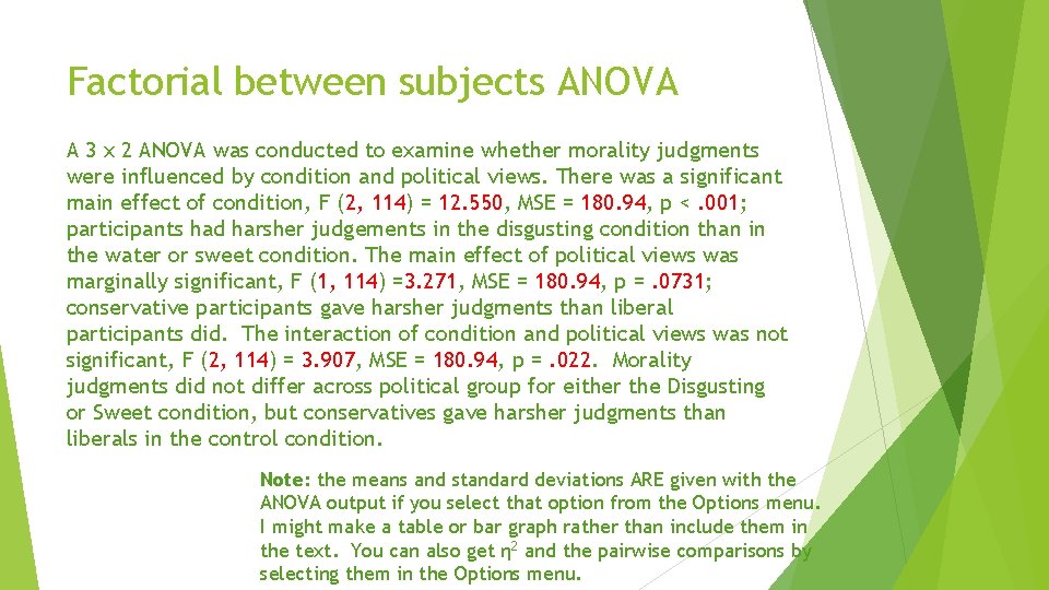
Factorial between subjects ANOVA A 3 x 2 ANOVA was conducted to examine whether morality judgments were influenced by condition and political views. There was a significant main effect of condition, F (2, 114) = 12. 550, MSE = 180. 94, p <. 001; participants had harsher judgements in the disgusting condition than in the water or sweet condition. The main effect of political views was marginally significant, F (1, 114) =3. 271, MSE = 180. 94, p =. 0731; conservative participants gave harsher judgments than liberal participants did. The interaction of condition and political views was not significant, F (2, 114) = 3. 907, MSE = 180. 94, p =. 022. Morality judgments did not differ across political group for either the Disgusting or Sweet condition, but conservatives gave harsher judgments than liberals in the control condition. Note: the means and standard deviations ARE given with the ANOVA output if you select that option from the Options menu. I might make a table or bar graph rather than include them in the text. You can also get η 2 and the pairwise comparisons by selecting them in the Options menu.

How to reports results from RCommander Finding Means and Standard Deviations Independent Paired samples t-test One-way ANOVA (RM ANOVA) Factorial ANOVA (RM Factorial ANOVA) Correlation Regression

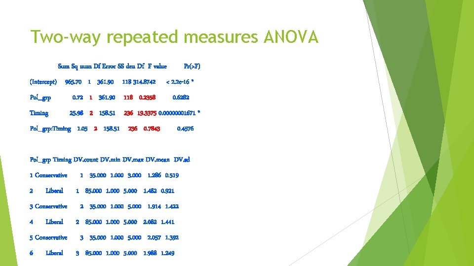
Two-way repeated measures ANOVA Sum Sq num Df Error SS den Df F value (Intercept) 965. 70 1 361. 90 118 314. 8742 Pr(>F) < 2. 2 e-16 * Pol_grp 0. 72 1 361. 90 118 0. 2358 0. 6282 Timing 25. 98 2 158. 51 236 19. 3375 0. 00000001671 * Pol_grp: Timing 1. 05 2 158. 51 236 0. 7843 0. 4576 Pol_grp Timing DV. count DV. min DV. max DV. mean DV. sd 1 Conservative 2 Liberal 3 Conservative 4 Liberal 5 Conservative 6 Liberal 1 35. 000 1. 000 3. 000 1. 286 0. 519 1 85. 000 1. 000 5. 000 1. 482 0. 921 2 35. 000 1. 000 5. 000 1. 914 1. 422 2 85. 000 1. 000 5. 000 2. 082 1. 441 3 35. 000 1. 000 5. 000 2. 057 1. 392 3 85. 000 1. 000 5. 000 1. 988 1. 249

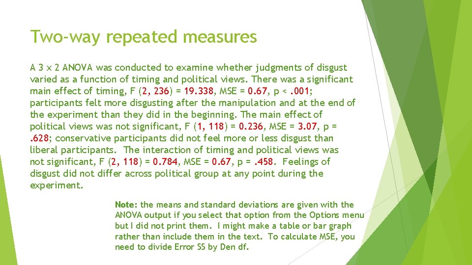
Two-way repeated measures A 3 x 2 ANOVA was conducted to examine whether judgments of disgust varied as a function of timing and political views. There was a significant main effect of timing, F (2, 236) = 19. 338, MSE = 0. 67, p <. 001; participants felt more disgusting after the manipulation and at the end of the experiment than they did in the beginning. The main effect of political views was not significant, F (1, 118) = 0. 236, MSE = 3. 07, p =. 628; conservative participants did not feel more or less disgust than liberal participants. The interaction of timing and political views was not significant, F (2, 118) = 0. 784, MSE = 0. 67, p =. 458. Feelings of disgust did not differ across political group at any point during the experiment. Note: the means and standard deviations are given with the ANOVA output if you select that option from the Options menu but I did not print them. I might make a table or bar graph rather than include them in the text. To calculate MSE, you need to divide Error SS by Den df.

How to reports results from RCommander Finding Means and Standard Deviations Independent Paired samples t-test One-way ANOVA (RM ANOVA) Factorial ANOVA (RM Factorial ANOVA) Correlation Regression

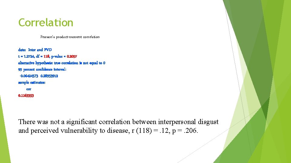
Correlation Pearson's product-moment correlation data: Inter and PVD t = 1. 2724, df = 118, p-value = 0. 2057 alternative hypothesis: true correlation is not equal to 0 95 percent confidence interval: -0. 06424573 0. 28953912 sample estimates: cor 0. 1163353 There was not a significant correlation between interpersonal disgust and perceived vulnerability to disease, r (118) =. 12, p =. 206.

How to reports results from RCommander Finding Means and Standard Deviations Independent Paired samples t-test One-way ANOVA (RM ANOVA) Factorial ANOVA (RM Factorial ANOVA) Correlation Simple Regression / Multiple Regression

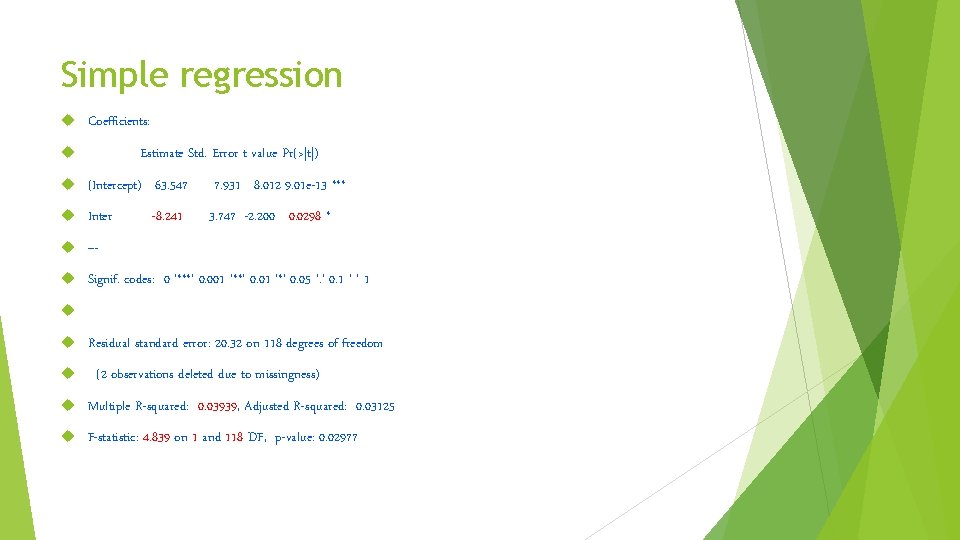
Simple regression Coefficients: Estimate Std. Error t value Pr(>|t|) (Intercept) 63. 547 7. 931 8. 012 9. 01 e-13 *** Inter 3. 747 -2. 200 0. 0298 * --- Signif. codes: 0 '***' 0. 001 '**' 0. 01 '*' 0. 05 '. ' 0. 1 ' ' 1 Residual standard error: 20. 32 on 118 degrees of freedom -8. 241 (2 observations deleted due to missingness) Multiple R-squared: 0. 03939, Adjusted R-squared: 0. 03125 F-statistic: 4. 839 on 1 and 118 DF, p-value: 0. 02977

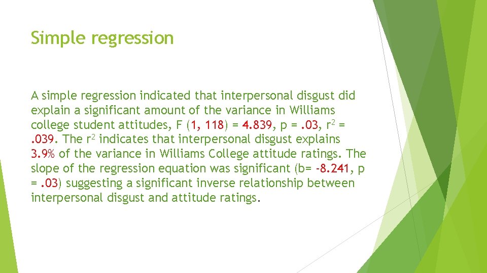
Simple regression A simple regression indicated that interpersonal disgust did explain a significant amount of the variance in Williams college student attitudes, F (1, 118) = 4. 839, p =. 03, r 2 =. 039. The r 2 indicates that interpersonal disgust explains 3. 9% of the variance in Williams College attitude ratings. The slope of the regression equation was significant (b= -8. 241, p =. 03) suggesting a significant inverse relationship between interpersonal disgust and attitude ratings.

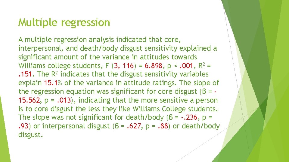
Multiple regression Coefficients: Estimate Std. Error t value Pr(>|t|) (Intercept) 87. 3278 9. 7917 8. 919 8. 05 e-15 *** Core 4. 3489 -3. 578 0. 000506 *** -15. 5615 Death. Body -0. 2358 Inter 0. 6266 2. 8328 -0. 083 0. 933800 4. 2524 0. 147 0. 883118 --Signif. codes: 0 '***' 0. 001 '**' 0. 01 '*' 0. 05 '. ' 0. 1 ' ' 1 Residual standard error: 19. 26 on 116 degrees of freedom Multiple R-squared: 0. 1514, Adjusted R-squared: 0. 1294 F-statistic: 6. 898 on 3 and 116 DF, p-value: 0. 0002579

Multiple regression A multiple regression analysis indicated that core, interpersonal, and death/body disgust sensitivity explained a significant amount of the variance in attitudes towards Williams college students, F (3, 116) = 6. 898, p <. 001, R 2 =. 151. The R 2 indicates that the disgust sensitivity variables explain 15. 1% of the variance in attitude ratings. The slope of the regression equation was significant for core disgust (β = 15. 562, p =. 013), indicating that the more sensitive a person is to core disgust the less they like Williams College students. The slope was not significant for death/body (β = -. 236, p =. 93) or interpersonal disgust (β =. 627, p =. 88) or death/body disgust.