Recent Developments in Inverse Scattering for Maxwells Equations


 Incomplete or")


 ill-posed: Alessandrini’ 87, Mandache’ 01")


 1")
 PML was first proposed by Berenger in 1994 as an")
")
 Consider the PML in spherical coordinates for")


 or near-field (subwavelength) Multiple frequency data")

 Recently, it is confirmed that the loss is related to the nonradiative")

,")


 In short")


 and the reconstruction (bottom) with full aperture data Slice x")
 and the reconstruction (bottom) with limited aperture data Slice x")


 Inverse Source Problems (joint with Lin & Triki, JDE, 2010) Linear but with")
 S is compactly")

 Assume that (1) The support volume (2)")
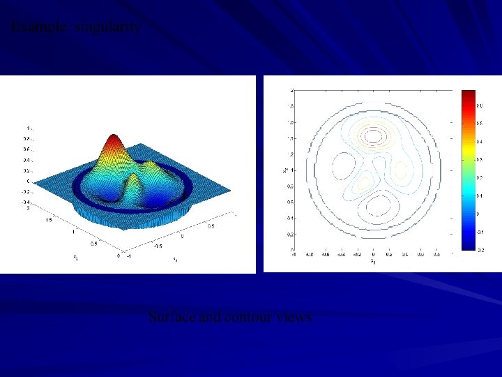
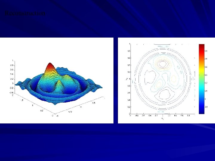
 (b) Fig 1. Surface and contour plots of the real source")
 (b) (c) Fig 3. Image of the real source solution (a); and reconstructed")
 random medium Determination")
")
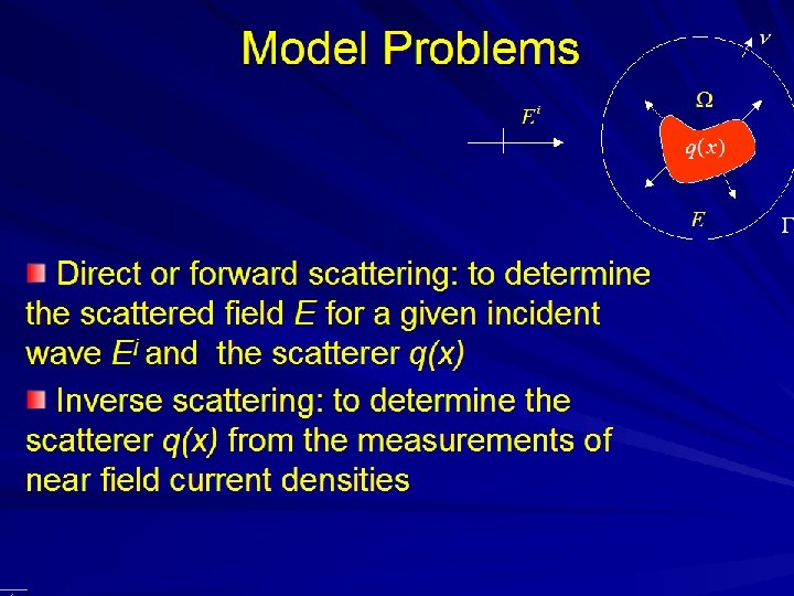
 Inverse scattering by near-field measurements Scattered field Radiation condition Boundary condition Inverse Problem:")
 well-posedness study of the forward problem. G. Derveaux, G.")


 Applications areas:")


- Slides: 75
Recent Developments in Inverse Scattering for Maxwell's Equations and Applications Gang Bao Interdisciplinary Center for Appl. & Comput. Math, Zhejiang U Michigan Center for Industrial & Applied Math, Michigan State U
Acknowledgements Collaborators: Peijun Li, Ying Li, Junshan Lin, Hai Zhang Faouzi Triki, Mickey S. Hou, Ki. Hyun Yun S-N Chow, H-M Zhou, J. Zou Research supported in parts by: NSF Appl. /Comput. Math. Programs NSF Theoretical Foundation Programs NSF Collaboration in Math. & Geo. Science Programs NSF Focused Research Group Programs Office of Naval Research Applied Analysis Programs
Outline Motivation and problem formulation Ill-posedness for inverse BVP Inverse scattering for Maxwell’s equations: multiple frequency data, convergence Inverse source problems Ongoing and future research
3 -D Inverse Medium Scattering Applications Non-destructive testing, material characterization and design Ultra sound tomography Seismic imaging Submarine detection Remote sensing Near-field and nano optics, diffraction limit, super-resolution, nano-technology
Inverse Boundary Value Problems: Challenges Nonlinear, ill-posedness, global versus local (initial guess) Incomplete or partial data Uncertainty, indistinguishability Large-scale computation: complexity, iterative, memory, CPU, choice of methods Stochastic versus deterministic
Inverse Scattering in Complex Media Stochastics Applications in sensing Raman spectroscopy for bio and environmental sensing Photonic Crystal spectrometer (in nano-scale) Human tissue Spatially incoherent light
Inverse Boundary Value Problems: theory The inverse conductivity problem: Calderon’s Problem: To determine the conductivity function from the boundary data (Dt. N or voltage to current map) Ref: On an inverse boundary value problem, in ``Seminar on Numerical Analysis and its Applications to Continuum Physics’’, pp. 65 -73, Soc. Brasilerira de Matematica, Rio de Haneiro, 1980 Calderon, Kohn-Vogelius, Uhlmann-Sylvester, Nachman, Isakov, Alessandrini, …. (Uniqueness and stability)…
Inverse Boundary Value Problems: Good News Lots of results, extensions: Sylvester & Uhlmann 1987 , Ann. Math. 125 Nachman 1988 , Ann. Math. 128 Nachman 1995, Ann. Math. 142 Pestov & Uhlmann 2005 , Ann. Math. (2) 161 Kari Astala and Lassi Päivärinta 2006, Ann. Math. 163 Kenig, Sjöstrand, & Uhlmann 2007, Ann. Math. (2)165 EIT: algorithms…
Inverse Boundary Value Problems: Bad News Ill-posedness Severely (exponentially) ill-posed: Alessandrini’ 87, Mandache’ 01 More questions than answers! Various means to overcome the ill-posedness: Seo, Nachman, … What is wrong? ! More data…
Objective To develop a data driven reconstruction method for solving the inverse problems. Objective: Stable reconstruction methods Engineering practice: broad band data, frequency sweeping. Some hints from the corresponding hyperbolic inverse problems: B. & Yun (2008) (also Sun ’ 90, Alessandrini &Sylvester ’ 90)
Scattering Model: Maxwell’s Equations in Unbounded Domains Boundary conditions Regularity analysis Numerical solution Refs: Muller (1969) , Abboud and Nedelec (1992), Costabel (1991), Birman and Solomyak (1987), Leis (1986), Kirsch and Monk (1995, 1998) Lp estimates, B. , Minut, Zhou (CPDE, 2007) B. , Li, Zhou (JDE, 2008)
Scattering: Time Hramonic Maxwell’s Equations Where Ei is the incident field E is the scattered field
Artificial Boundary Conditions Absorbing boundary conditions Transparent boundary conditions Perfectly matched layers (PML) 1 st order absorbing boundary condition
Perfectly Matched Layers (PML) PML was first proposed by Berenger in 1994 as an artificial boundary layer for Maxwell equations on unbounded domains The idea is to surround the computational domain by a nonphysical so called PML medium which can absorb without reflection outgoing waves of any frequency or any incident direction; the waves decay exponentially into the PML medium.
PML: Issues In practice, the PML medium must be truncated and the new (PML) boundary generates reflected waves which can pollute the solution in the computational domain. Error estimates in the computational domain between the solutions of the original scattering and the truncated PML problems. Related works: Helmholtz scattering problems: Lassas and Somersalo (98, 01), Hohage, Schmidt, and Zschiedrich (2001), Chen and Liu (2005). 3 -D EM scattering: little is known!
PML Analysis (B. & Wu, SINA 05) Consider the PML in spherical coordinates for 3 -D EM scattering. Under the well-posedness assumption of the original scattering problem: (spherical harmonics!) the truncated PML problem attains a unique solution in the PML solution converges exponentially toward the scattering solution in the computational domain when either the PML medium parameter or the layer thickness is increased. the error estimate is explicit and may be used to determine the PML medium parameter.
Variational Problem
Compact Imbedding
More General Scattering Model Consider the following general form: With jump coefficients and smooth interfaces Applications include: Modeling of nonlinear optics Scattering by nonlinear media
Interior Regularity Theorem: For Then for Let
Global Estimates Interior estimates. Boundary estimates: a new version of Maximum Principle. Decompose the fields into propagating modes and evanescent modes Scattering by periodic structures (B. , Minut, and Zhou, CPDE ‘ 07) and general bounded media (B. , Li, Zhou, JDE, ‘ 08) Many open problems!
3 -D Inverse Medium Scattering To reconstruct the medium from boundary easurements: Dorn, Bertete-Aguirre, Berryman, Papanicolaou (1999), Haddar and Monk (2002), Hohage (2003), Colton and Kress, W. Chew et al (2003, 2004) Theoretical studies…: Dt. N data
Measured Data Boundary measurements: far-field (a few wavelength) or near-field (subwavelength) Multiple frequency data Fixed frequency Incomplete or partial data A reconstruction should be no more precise than that the data it represents.
Uncertainty Principle At the end of 19 th century, Abbe and Rayleigh showed: there is a limit to the sharpness of details that could be observed by an optical microscope Heisenberg later used the optical experiment to illustrate that the smallest details of the medium that can be detected are always larger than a half wavelength! Far field versus near-field!
Uncertainty Principle(cont’d) Recently, it is confirmed that the loss is related to the nonradiative components of the field -- evanescent waves confined on the surface of the scatterer (a few nanometers) and decaying outside the smallest distance between two solved points in the spatial or frequency domain, and the approximate spread in wave number Good news: It does not limit the resolution rather offers a limit on the accuracy of the reconstruction at a given wave number. To increase the resolution, a larger wave number is
Reconstruction via Uncertainty Principle The Uncertainty Principle in inverse medium scattering:
Continuation Method 2 -D Inverse medium scattering – Full aperture, Chen & Rokhlin (97), Chen (97 a, 97 b), Analysis, B. , Chen, & Ma(00) – Limited aperture, B. & Liu (03), B. & Li (07) – Fixed frequency, B. & Li (05, 06, 07) – Convergence, B. & Triki (08) Inverse obstacle scattering problem – Coifman, Goldberg, Hrycak, & Rokhlin (99) – B. , Hou, & Li (07) 3 -D Inverse medium scattering problem
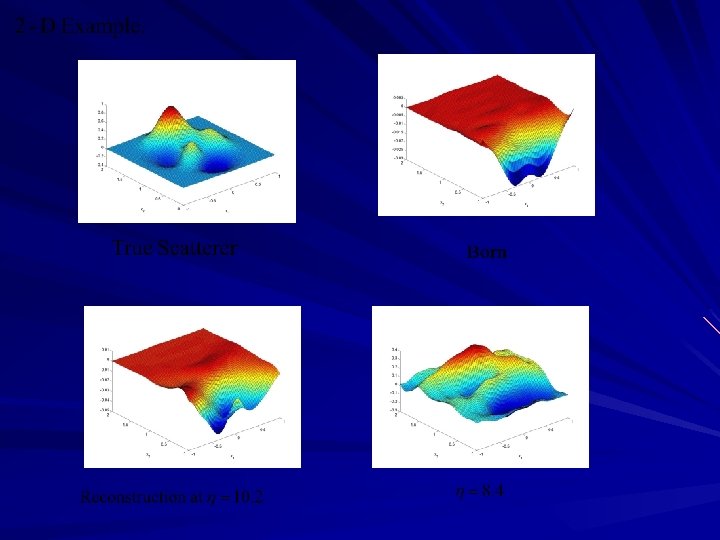
Weak Scattering The nonlinear relation between E and q is essentially linear if one of the following conditions is satisfied: • q small • k small • small Weak scattering:
Low Frequency Modes Integration by parts Linearization
Kaczmarz method (Natterer, 86) In short
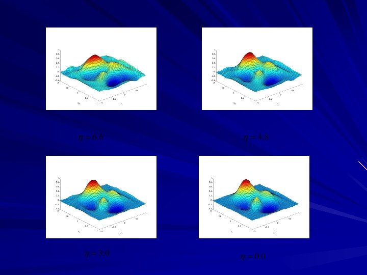
Recursive Linearization
Backprojection regularization
Adjoint State Method
Reconstruction Algorithm: Beyond Born
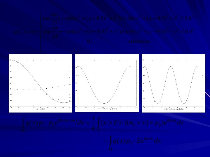
Numerical Experiments Forward solver: 2 nd order symmetric Edge Element for tetrahedral, reverse Cuthill-Mc. Kee (RCM) ordering, compressed row storage (CRS), Bi. Conjugate Gradient (Bi. CG) and Quasi-Minimal Residual (QMR) with diagonal preconditioning
Numerical Experiments Forward solver: 2 nd order symmetric Edge Element for tetrahedral, reverse Cuthill-Mc. Kee (RCM) ordering, compressed row storage (CRS), Bi. Conjugate Gradient (Bi. CG) and Quasi-Minimal Residual (QMR) with diagonal preconditioning
k 1 2 3 4 5 6 7 e 2 0. 839 0. 783 0. 703 0. 644 0. 506 0. 362 0. 293
Recursive Linearization for Fixed Frequency IMP: Evanescent Incident Fields Choose a large spatial frequency parameter Divide the interval Computer the initial guess via Born (weak scattering) Recursive linearization Subwavelength resolution
Incidence Plane Waves
The true scatterer (top) and the reconstruction (bottom) with full aperture data Slice x 1=0. 3 Slice x 2=0 Slice x 3=0
The true scatterer (top) and the reconstruction (bottom) with limited aperture data Slice x 1=0. 3 Slice x 2=0 Slice x 3=0
Convergence Analysis Objective: to explain excellent numerical results in 2 -D and 3 -D cases. Idea: Uncertainty principle, B. & Triki (08) Theorem:
Convergence Analysis: Discussions Linear convergence as the wave number goes to the infinity For a bounded sequence of wave numbers convergence to the observable part of the medium The regularization parameter indicates the computational cost How certain is Uncertainty Principle ? ? ?
General Remarks A continuation method based on uncertain principle has been developed. The approach is physically motivated with data driven accuracy -- it leads to the reconstruction allowed by the measured data but nothing more! The method is accurate, which is consistent with the underlying physics. Our convergence analysis confirms the excellent numerical results by taking into account of the uncertainty principle.
(II) Inverse Source Problems (joint with Lin & Triki, JDE, 2010) Linear but with many common features Complete stability analysis with fixed frequency or multiple frequency data; Promising numerical results Previous results: Bleistein & Cohen`77, He & Romanov`98, Ammari, B. , Fleming `02; Albanese&Monk `06, Davaney et al `04, 07 Difficulties: Nonuniqueness and ill-posedness.
Consider reconstruction of the source function for the Helmholtz Equation (1) S is compactly supported with support volume (2) Multi-frequency data are measured on ISP: to reconstruct S from multi-frequency data. ,
Uniqueness Theorem Let be a bounded and a strictly monotone sequence. Then the measurements uniquely determines the source function S. Stability Estimates 1 (size of is fixed) Assume that (1) The support volume (2) , ; . Two constants Then (a). If , (b). If , ; .
Stability Estimates 2 ( is fixed, ) Assume that (1) The support volume (2) ; , , . Two constants (3) Then (a). If (b). If , ; , .
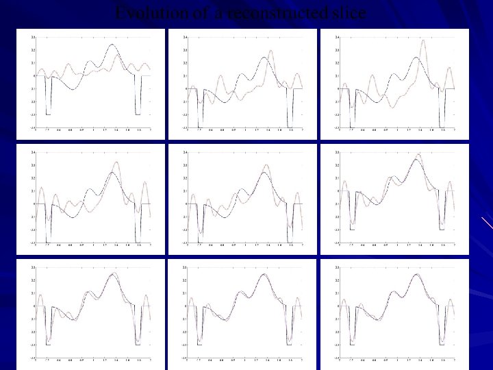
Numerical Examples (a) (b) Fig 1. Surface and contour plots of the real source function (a); and the reconstruction (b) at k=61. Fig 2. Evolution of the reconstructions at k = 9, 17, 25 (Top, left to right), 33, 41, 61 (Bottom, left to right).
(a) (b) (c) Fig 3. Image of the real source solution (a); and reconstructed solution (b) with 10% noise in measurements; (c) is the image of the numerical error. , wavelength , the distance between two discs is.
Inverse Source Problems Limited aperture Inhomogeneous media ISP in a (weakly) random medium Determination of a stochastic source Cloak a source?
Concluding Remarks:Stability Calderon’s problem: bad/optimal estimate Almost Lipschitz type estimate (B. & Yun’ 08) Velocity inversion? Estimates for the multiple frequency case --completely open for inverse medium problem! ISP Convergence study of recursive linearization --- rigorous characterization of the uncertainty principle
(III) Inverse scattering by near-field measurements Scattered field Radiation condition Boundary condition Inverse Problem: For near-field measurement reconstruct from on the plane , .
Recent studies A. Willers, (1987) well-posedness study of the forward problem. G. Derveaux, G. Papanicolaou and C. Tsogka, (2006) linearized model ( ), denoising using broadband signals. S. Chandler-wilde et al, scattering by unbounded rough surface. H. Ammari, G. Bao, A. Wood, analysis of the cavity problem (local downward surface displacement) Challenges : nonlinearity, ill-posedness,diffraction limit Opportunity : evanescent mode becomes significant in near field regime.
Analysis of the scattered wave Boundary integral formulation: Plane wave decomposition of Green’s function where Scattered field consists of propagation and evanescent mode!
Analysis of the scattered wave Fourier domain: if where High spatial frequency component of scattered field (evanescent mode) carries high spatial frequency information of the surface. Near-field versus Far-field: (1) Evanescent modes are not accessible in far field-regime, while significant in near-field regime! (2) Evanescent modes make it possible to break the diffraction limit.
Reconstruction procedure Step 1: Let where Near-field versus Far-field: Step 2: Correction of on the boundary Step 3: Match the data on the surface:
Numerical example for 2 d problem Wavenumber k=100, normal incidence Near field reconstruction, measurement distance: The distance between two bumps: . super resolution is achieved! without noise 5% additive noise Far-field reconstruction, measurement distance:
Near-Field Imaging: to break the diffraction limit Real profile, the distance between neighboring bumps is Comparison of the reconstruction (5% additive noise in measurement) with the real profile for the near field case.
Incomplete or Partial Data Limited aperture Phaseless data Poor initial guess Mathematical issues: to redefine uniqueness & stability
Inverse Backscattering with Limited Aperture Data
Inverse Scattering in Complex Media Dispersive Medium Applications include breast cancer detections and imaging of human tissues Multi-frequency data but the dielectric coefficients (medium) are now frequency dependent: the Debye model To determine two functions instead of one! Large scale inverse problems
Inverse Scattering in Complex Media Stochastics Applications in sensing Raman spectroscopy for bio and environmental sensing Photonic Crystal spectrometer (in nano-scale) Human tissue Spatially incoherent light
Micro Diffractive Optics Maxwell’s Eqns in periodic complicated media (optical diffraction gratings) Applications areas: optical comm. , optical storage, sensors, displays, corrective lenses, scanners, laser technology, security, … Optical medium: --- Classical --- Chiral --- Nonlinear: second harmonic generation --- Anisotropic Issues: Modeling, simulation, analysis, & optimal design
Computational Modeling of Optical Response from Excitons in Nano Media Excitons confined in a nano-scale medium. Semiclassical Model: Maxwell’s Eqs. + Schroedinger Eqs. Dielectric constant: (Derived from first principle)
1 -D and 2 -D confinements Helmholtz equation: Dispersion relation: gives two modes Maxwell’s boundary conditions & additional boundary conditions are required ! ABC: Polarization induced by excitons vanish at the boundaries.
Nano Optical Modeling/Imaging ● An emerging area in optical science dealing with scales small but not yet atomic ● Microscopic versus macroscopic Maxwell’s equations ● Multiscale approaches are essential Long term objective: characterizations of nano materials/structures Other related topics: Uniqueness for IPs with minimum amount of data: 3 -D gratings (joint with Zhang, and Zou, TAMS) Stability estimates for high wave number problems (joint with Yun, Zhou)