Particle Filters Outline 1 Introduction to particle filters

Particle Filters

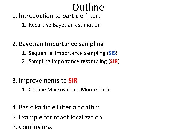
Outline 1. Introduction to particle filters 1. Recursive Bayesian estimation 2. Bayesian Importance sampling 1. Sequential Importance sampling (SIS) 2. Sampling Importance resampling (SIR) SIR 3. Improvements to SIR 1. On-line Markov chain Monte Carlo 4. Basic Particle Filter algorithm 5. Example for robot localization 6. Conclusions

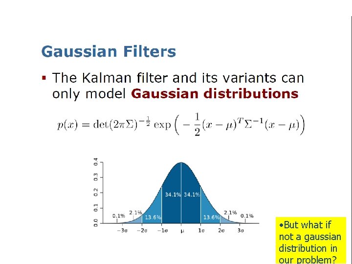
• But what if not a gaussian distribution in our problem?

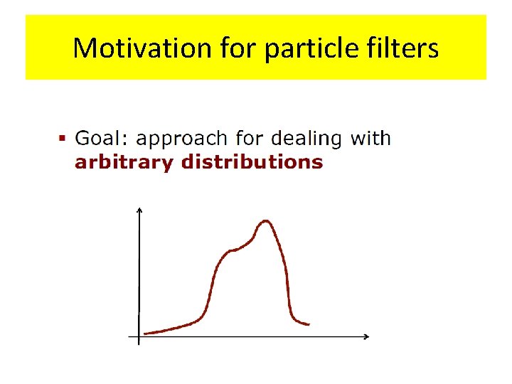
Motivation for particle filters

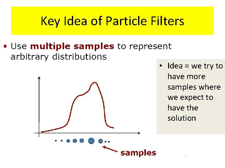
Key Idea of Particle Filters • Idea = we try to have more samples where we expect to have the solution

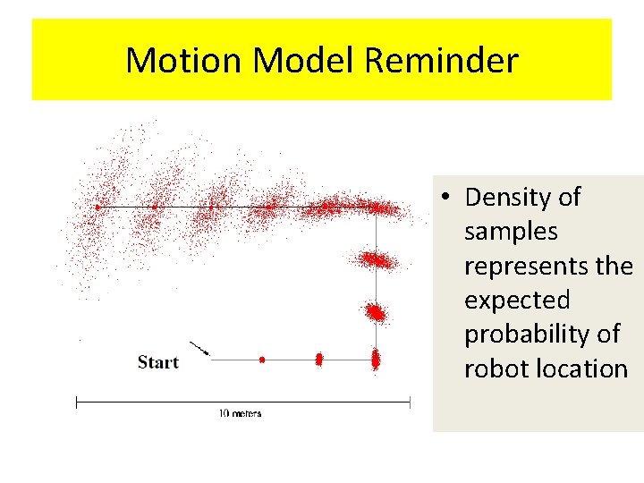
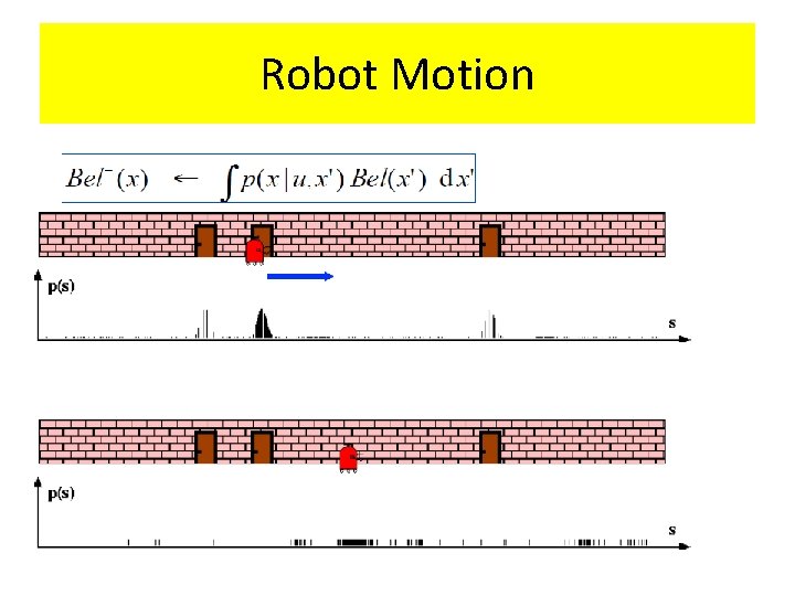
Motion Model Reminder • Density of samples represents the expected probability of robot location

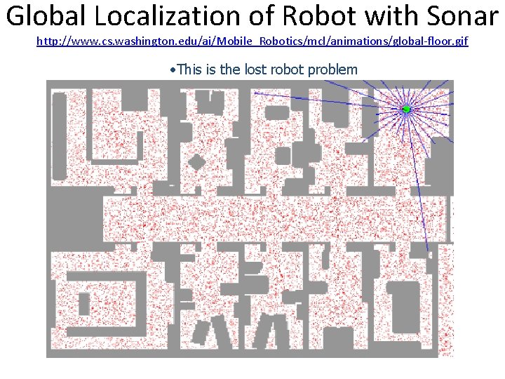
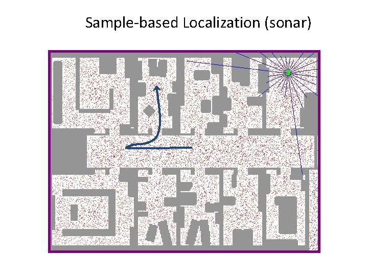
Global Localization of Robot with Sonar http: //www. cs. washington. edu/ai/Mobile_Robotics/mcl/animations/global-floor. gif • This is the lost robot problem

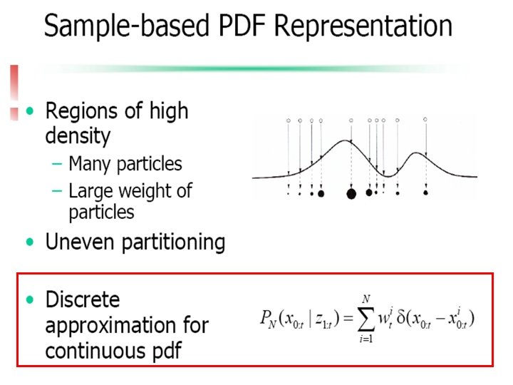
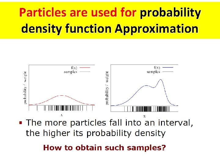
Particles are used for probability density function Approximation

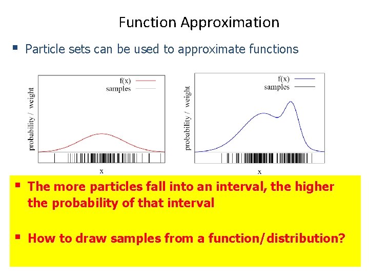
Function Approximation § Particle sets can be used to approximate functions § The more particles fall into an interval, the higher the probability of that interval § How to draw samples from a function/distribution?

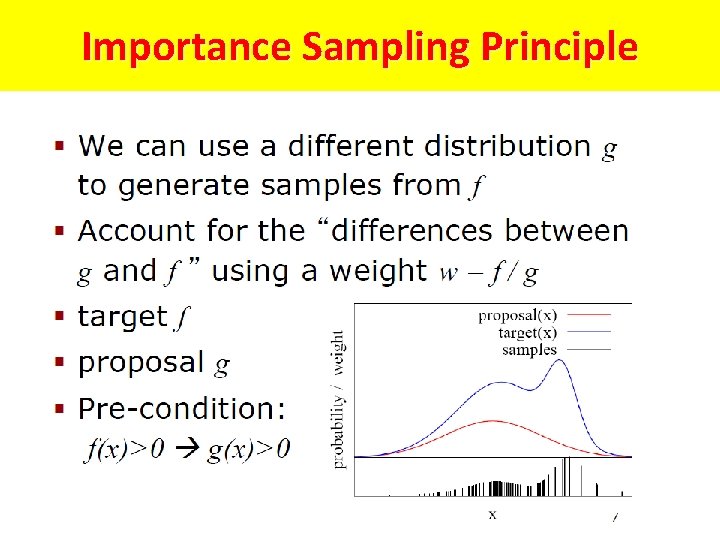
Importance Sampling Principle

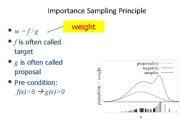
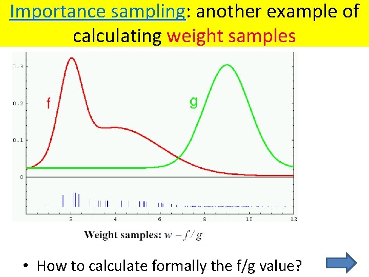
Importance Sampling Principle § w=f/g § f is often called target § g is often called proposal § Pre-condition: f(x)>0 g(x)>0 weight

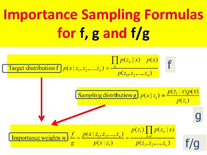
Importance sampling: sampling another example of calculating weight samples • How to calculate formally the f/g value?

Importance Sampling Formulas for f, g and f/g f g f/g

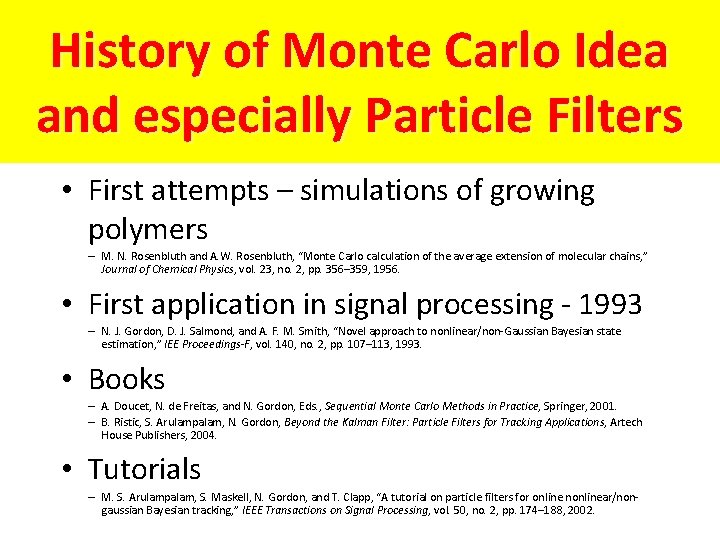
History of Monte Carlo Idea and especially Particle Filters • First attempts – simulations of growing polymers – M. N. Rosenbluth and A. W. Rosenbluth, “Monte Carlo calculation of the average extension of molecular chains, ” Journal of Chemical Physics, vol. 23, no. 2, pp. 356– 359, 1956. • First application in signal processing - 1993 – N. J. Gordon, D. J. Salmond, and A. F. M. Smith, “Novel approach to nonlinear/non-Gaussian Bayesian state estimation, ” IEE Proceedings-F, vol. 140, no. 2, pp. 107– 113, 1993. • Books – A. Doucet, N. de Freitas, and N. Gordon, Eds. , Sequential Monte Carlo Methods in Practice, Springer, 2001. – B. Ristic, S. Arulampalam, N. Gordon, Beyond the Kalman Filter: Particle Filters for Tracking Applications, Artech House Publishers, 2004. • Tutorials – M. S. Arulampalam, S. Maskell, N. Gordon, and T. Clapp, “A tutorial on particle filters for online nonlinear/nongaussian Bayesian tracking, ” IEEE Transactions on Signal Processing, vol. 50, no. 2, pp. 174– 188, 2002.

What is the problem that we want to solve? • The problem is tracking the state of a system as it evolves over time • Sequentially arriving (noisy or ambiguous) observations • We want to know: Best possible estimate of the hidden variables

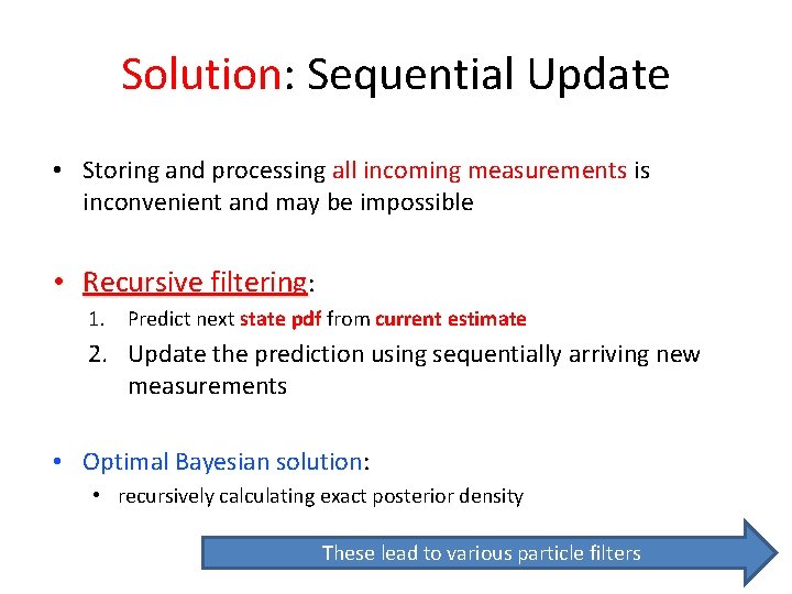
Solution: Sequential Update • Storing and processing all incoming measurements is inconvenient and may be impossible • Recursive filtering: 1. Predict next state pdf from current estimate 2. Update the prediction using sequentially arriving new measurements • Optimal Bayesian solution: solution • recursively calculating exact posterior density These lead to various particle filters

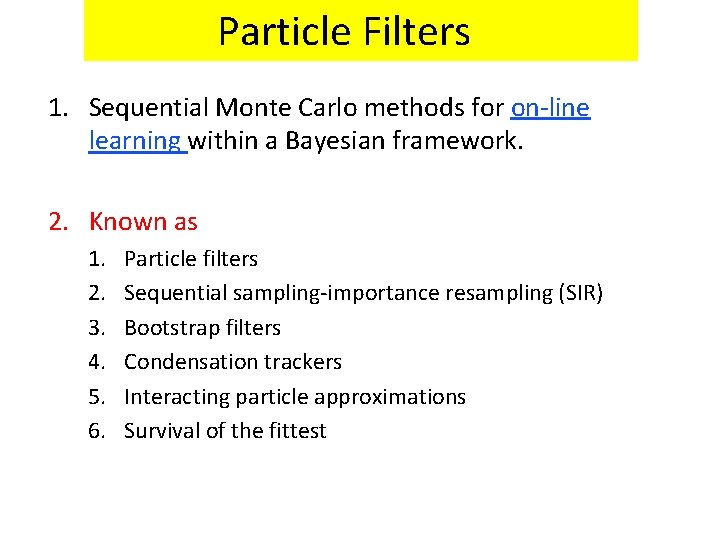
Particle Filters 1. Sequential Monte Carlo methods for on-line learning within a Bayesian framework. 2. Known as 1. 2. 3. 4. 5. 6. Particle filters Sequential sampling-importance resampling (SIR) Bootstrap filters Condensation trackers Interacting particle approximations Survival of the fittest

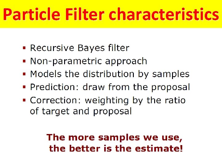
Particle Filter characteristics

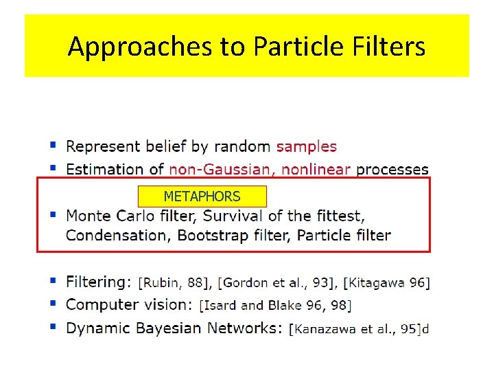
Approaches to Particle Filters METAPHORS

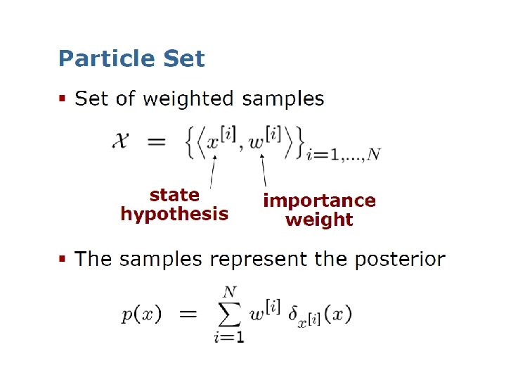
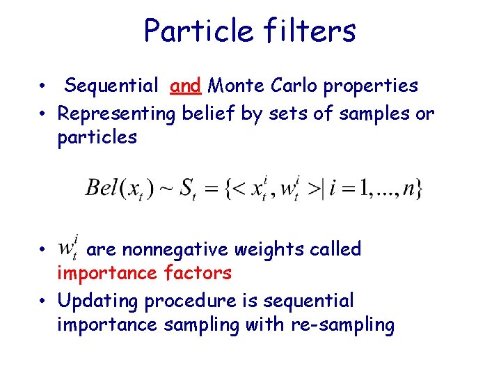
Particle filters • Sequential and Monte Carlo properties • Representing belief by sets of samples or particles are nonnegative weights called importance factors • Updating procedure is sequential importance sampling with re-sampling •

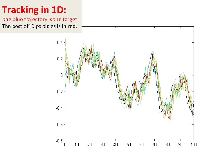
Tracking in 1 D: the blue trajectory is the target. The best of 10 particles is in red.

Short, more formal, Introduction to Particle Filters and Monte Carlo Localization

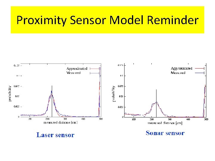
Proximity Sensor Model Reminder

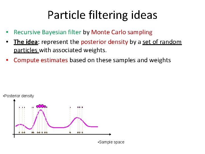
Particle filtering ideas • Recursive Bayesian filter by Monte Carlo sampling • The idea: idea represent the posterior density by a set of random particles with associated weights. • Compute estimates based on these samples and weights • Posterior density • Sample space

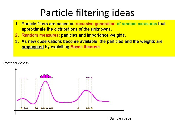
Particle filtering ideas 1. Particle filters are based on recursive generation of random measures that approximate the distributions of the unknowns. 2. Random measures: particles and importance weights. 3. As new observations become available, the particles and the weights are propagated by exploiting Bayes theorem • Posterior density • Sample space

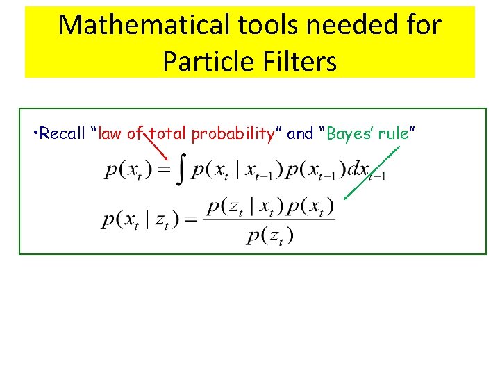
Mathematical tools needed for Particle Filters • Recall “law of total probability” and “Bayes’ rule”

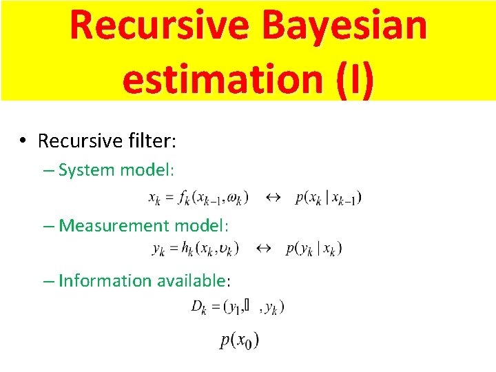
Recursive Bayesian estimation (I) • Recursive filter: – System model: – Measurement model: – Information available:

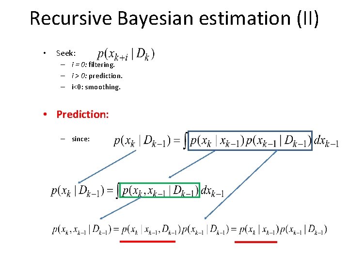
Recursive Bayesian estimation (II) • Seek: – i = 0: filtering. – i > 0: prediction. – i<0: smoothing. • Prediction: – since:

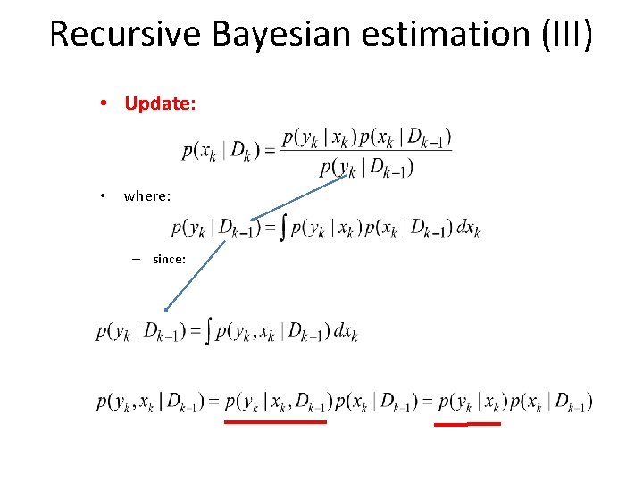
Recursive Bayesian estimation (III) • Update: • where: – since:

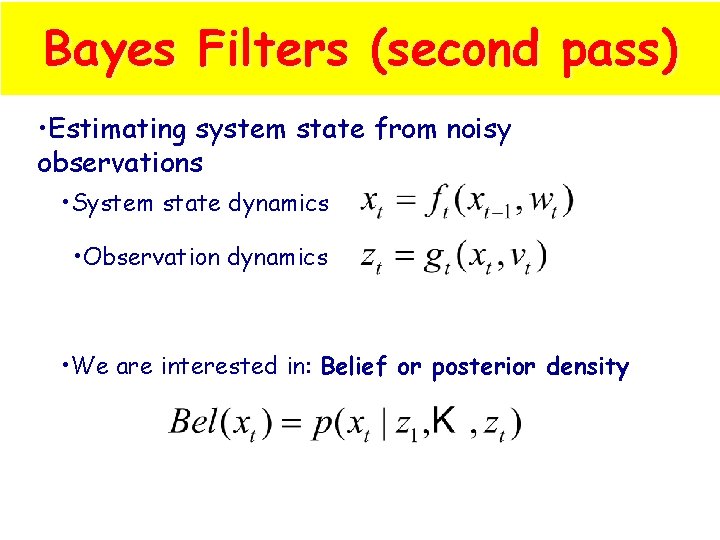
Bayes Filters (second pass) • Estimating system state from noisy observations • System state dynamics • Observation dynamics • We are interested in: Belief or posterior density

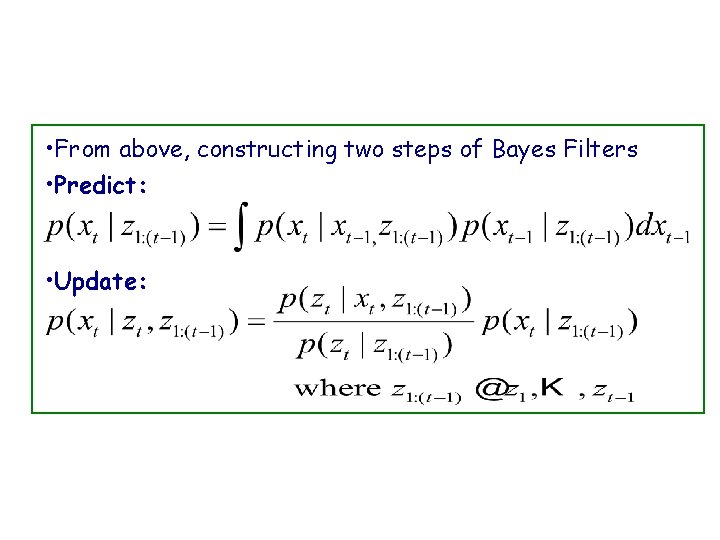
• From above, constructing two steps of Bayes Filters • Predict: • Update:

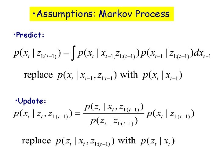
• Assumptions: Markov Process • Predict: • Update:

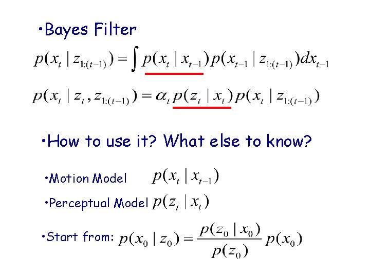
• Bayes Filter • How to use it? What else to know? • Motion Model • Perceptual Model • Start from:

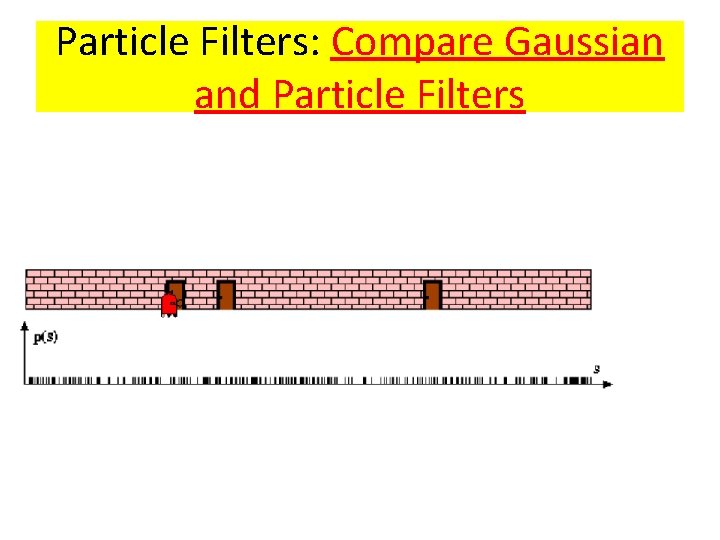
Particle Filters: Compare Gaussian and Particle Filters

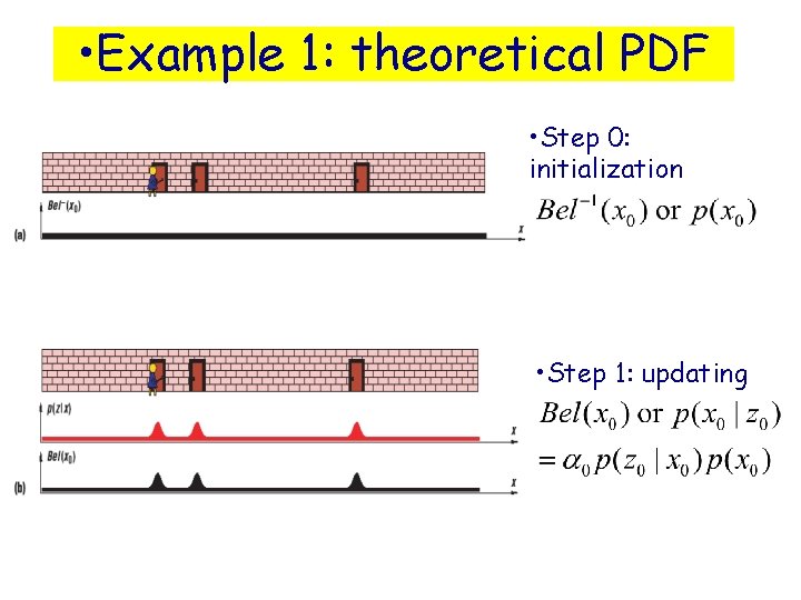
Example 1: theoretical PDF

• Example 1: theoretical PDF • Step 0: initialization • Step 1: updating

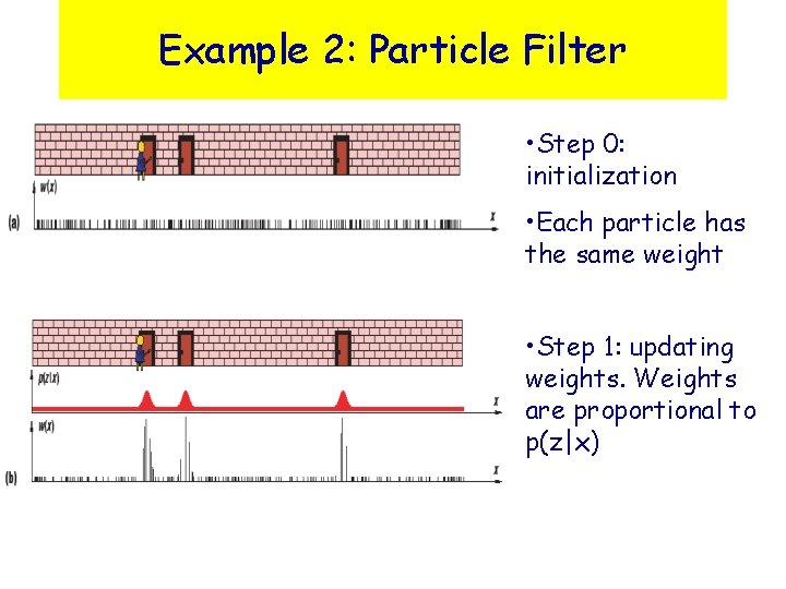
Example 2: Particle Filter • Step 0: initialization • Each particle has the same weight • Step 1: updating weights. Weights are proportional to p(z|x)

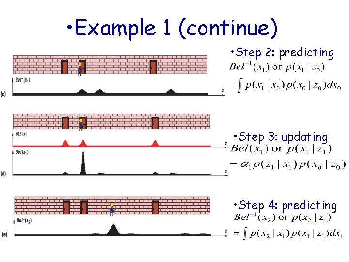
• Example 1 (continue) • Step 2: predicting • Step 3: updating • 1 • Step 4: predicting

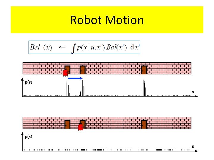
Robot Motion

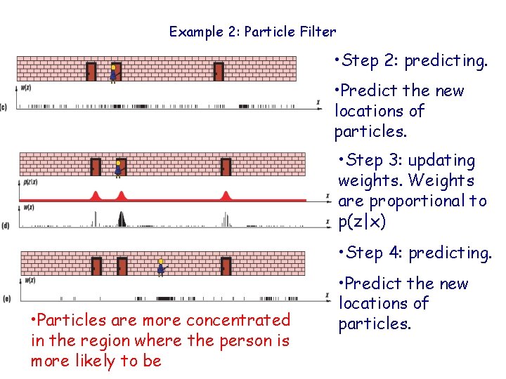
Example 2: Particle Filter

Example 2: Particle Filter • Step 2: predicting. • Predict the new locations of particles. • Step 3: updating weights. Weights are proportional to p(z|x) • Step 4: predicting. • Particles are more concentrated in the region where the person is more likely to be • Predict the new locations of particles.

Robot Motion

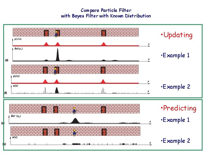
Compare Particle Filter with Bayes Filter with Known Distribution • Updating • Example 1 • Example 2 • Predicting • Example 1 • Example 2

Classical approximations • Analytical methods: – Extended Kalman filter, – Gaussian sums… (Alspach et al. 1971) • Perform poorly in numerous cases of interest • Numerical methods: – point masses approximations, – splines. (Bucy 1971, de Figueiro 1974…) • Very complex to implement, not flexible.

Monte Carlo Localization

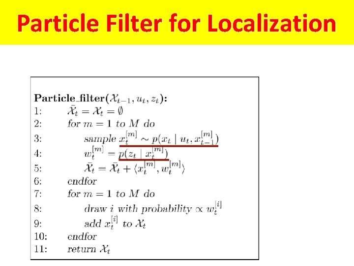
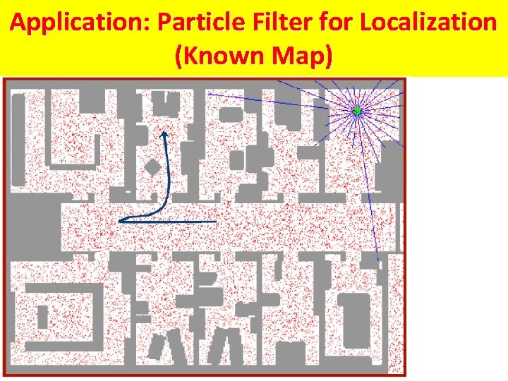
Mobile Robot Localization § Each particle is a potential pose of the robot § Proposal distribution is the motion model of the robot (prediction step) § The observation model is used to compute the importance weight (correction step)

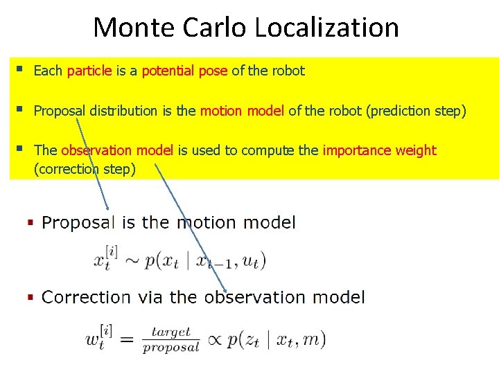
Monte Carlo Localization § Each particle is a potential pose of the robot § Proposal distribution is the motion model of the robot (prediction step) § The observation model is used to compute the importance weight (correction step)

Sample-based Localization (sonar)

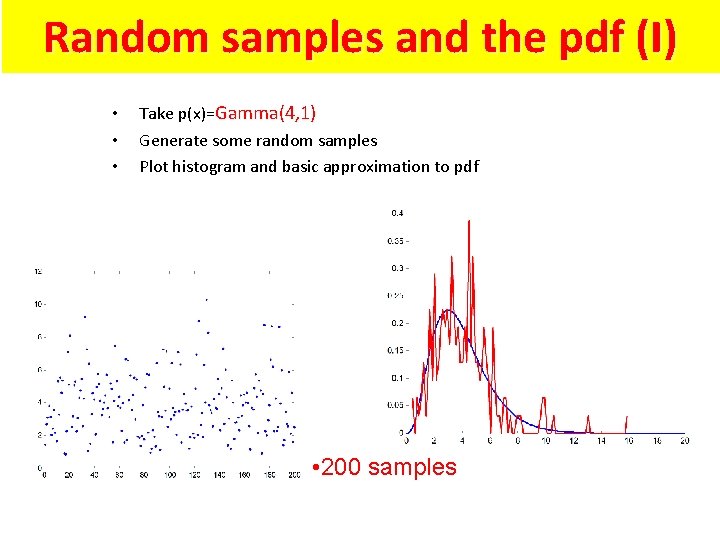
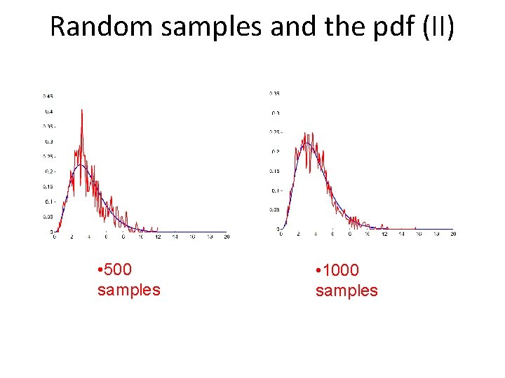
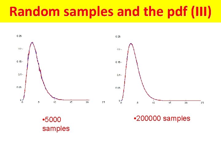
Random samples and the pdf (I) • • • Take p(x)=Gamma(4, 1) Generate some random samples Plot histogram and basic approximation to pdf • 200 samples

Random samples and the pdf (II) • 500 samples • 1000 samples

Random samples and the pdf (III) • 5000 samples • 200000 samples

Importance Sampling

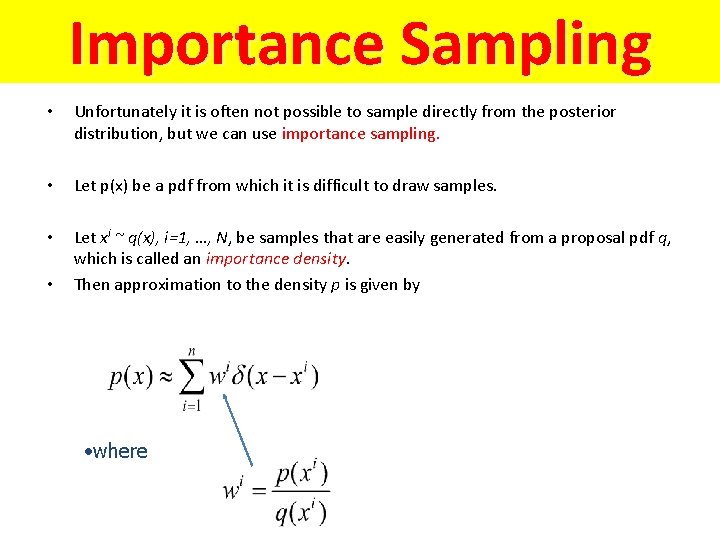
Importance Sampling • Unfortunately it is often not possible to sample directly from the posterior distribution, but we can use importance sampling. • Let p(x) be a pdf from which it is difficult to draw samples. • Let xi ~ q(x), i=1, …, N, be samples that are easily generated from a proposal pdf q, which is called an importance density. Then approximation to the density p is given by • • where

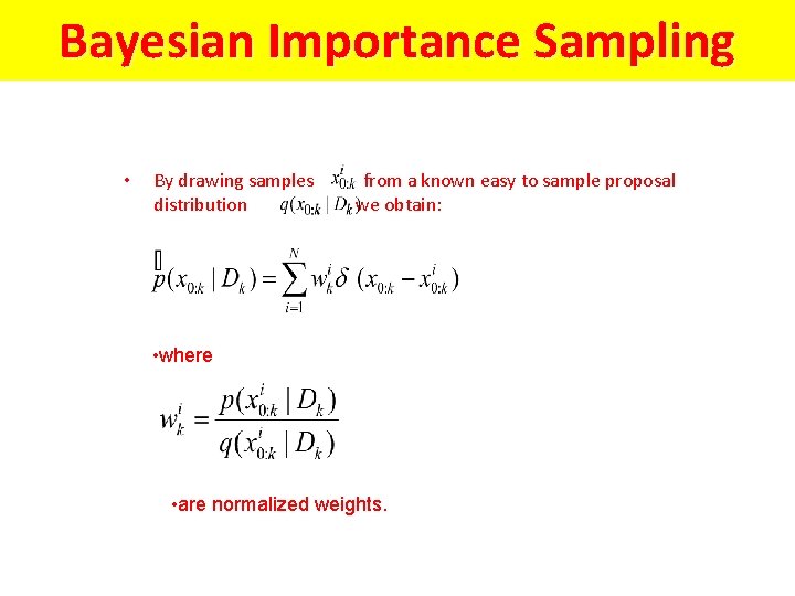
Bayesian Importance Sampling • By drawing samples distribution from a known easy to sample proposal we obtain: • where • are normalized weights.

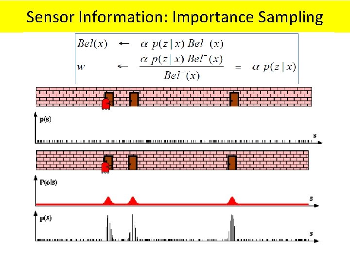
Sensor Information: Importance Sampling

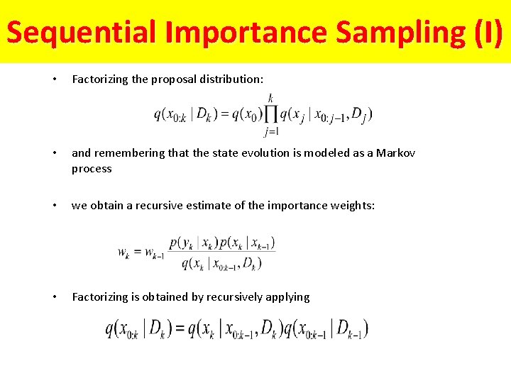
Sequential Importance Sampling (I) • Factorizing the proposal distribution: • and remembering that the state evolution is modeled as a Markov process • we obtain a recursive estimate of the importance weights: • Factorizing is obtained by recursively applying

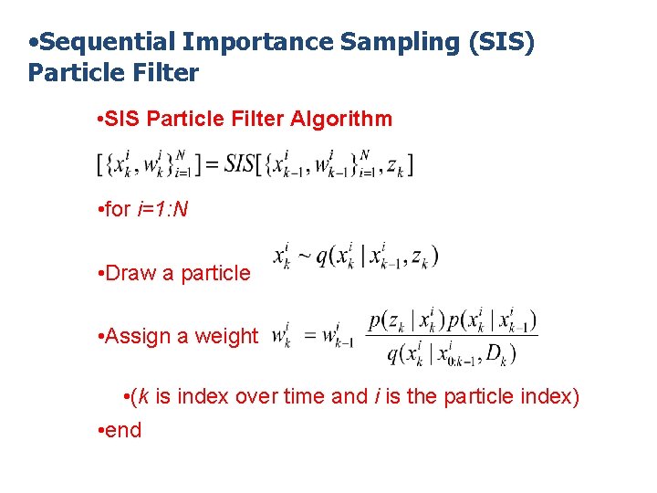
• Sequential Importance Sampling (SIS) Particle Filter • SIS Particle Filter Algorithm • for i=1: N • Draw a particle • Assign a weight • (k is index over time and i is the particle index) • end

Rejection Sampling

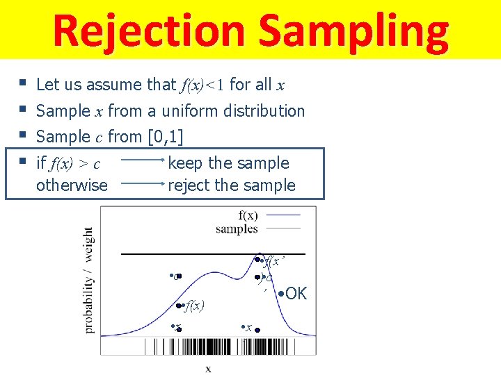
Rejection Sampling § § Let us assume that f(x)<1 for all x Sample x from a uniform distribution Sample c from [0, 1] if f(x) > c otherwise keep the sample reject the sample • f(x’ ) • c ’ • OK • c • f(x) • x ’

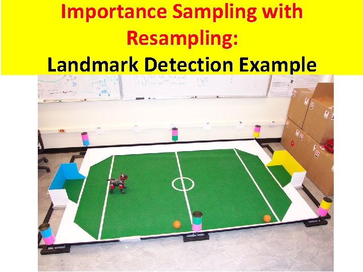
Importance Sampling with Resampling: Landmark Detection Example

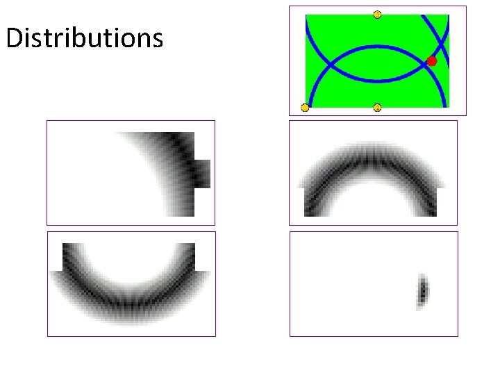
Distributions

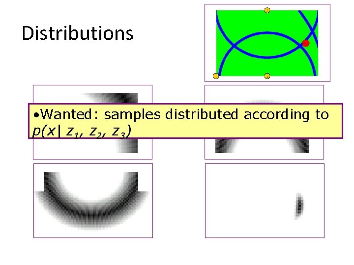
Distributions • Wanted: samples distributed according to p(x| z 1, z 2, z 3)

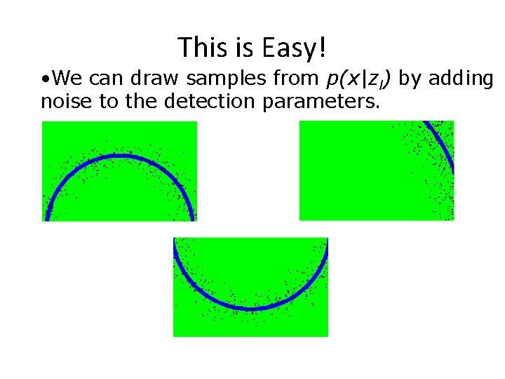
This is Easy! • We can draw samples from p(x|zl) by adding noise to the detection parameters.

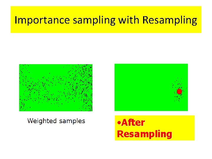
Importance sampling with Resampling • After Resampling

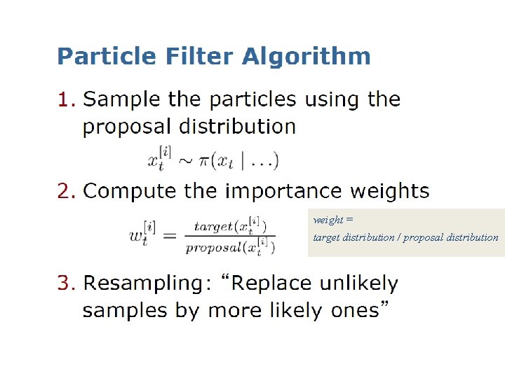
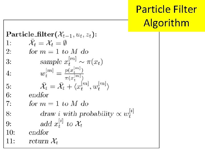
Particle Filter Algorithm

weight = target distribution / proposal distribution

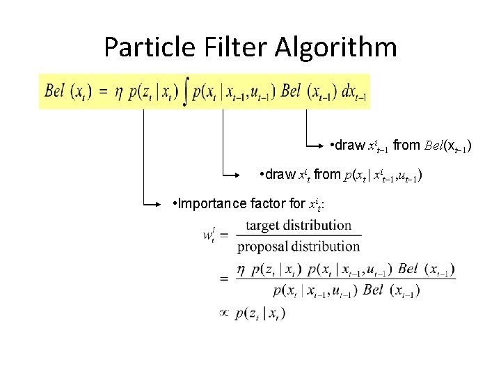
Particle Filter Algorithm • draw xit-1 from Bel(xt-1) • draw xit from p(xt | xit-1, ut-1) • Importance factor for xit:

Particle Filter Algorithm

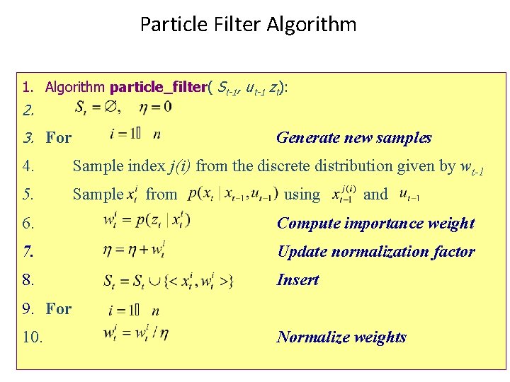
Particle Filter Algorithm 1. Algorithm particle_filter( St-1, ut-1 zt): 2. 3. For Generate new samples 4. Sample index j(i) from the discrete distribution given by wt-1 5. Sample from using and 6. Compute importance weight 7. Update normalization factor 8. Insert 9. For 10. Normalize weights

Particle Filter for Localization

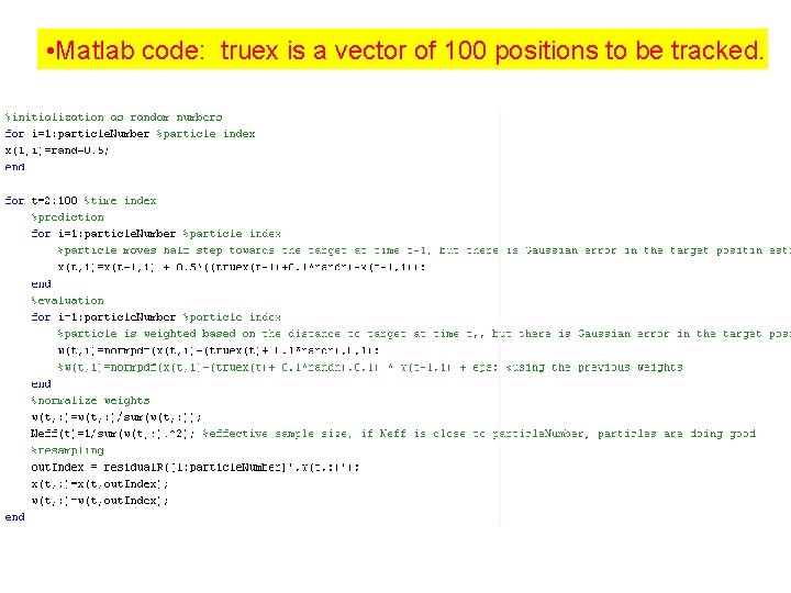
Particle Filter in Matlab

• Matlab code: truex is a vector of 100 positions to be tracked.

Application: Particle Filter for Localization (Known Map)

Sources • • • • Longin Jan Latecki Keith Copsey Paul E. Rybski Cyrill Stachniss Sebastian Thrun Alex Teichman Michael Pfeiffer J. Hightower L. Liao D. Schulz G. Borriello Honggang Zhang Wolfram Burgard Dieter Fox • • • Giorgio Grisetti Maren Bennewitz Christian Plagemann Dirk Haehnel Mike Montemerlo Nick Roy Kai Arras Patrick Pfaff Miodrag Bolic Haris Baltzakis • 76

77

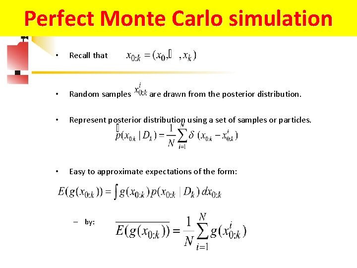
Perfect Monte Carlo simulation • Recall that • Random samples • Represent posterior distribution using a set of samples or particles. • Easy to approximate expectations of the form: – by: are drawn from the posterior distribution.