OneWay ANOVA I Class 17 Schedule for Remainder

One-Way ANOVA I Class 17

Schedule for Remainder of Semester 1. One way ANOVA 2. Two way ANOVA 3. Planned contrasts 4. Correlation and Regression 5. Moderated Multiple Regression 6. Survey design 7. Non-experimental designs IF TIME PERMITS 8. Writing up research Quiz 2: Nov. 12 -- up to and including one-way ANOVA Quiz 3: Dec. 5 – What we’ve covered by Dec. 3 Class Assignment: Assigned Nov. 26, Due Dec.

HANDS ON STATS PRACTICE SPSS Demo Tuesday, Nov. 12 2: 30 -3: 45 Location: Engelhard 309 NOTE: May change to Hill Hall 124, 12: 00 -2: 00 Homework: Extra Credit: 3 Pts full credit, 1 pt partial credit

ANOVA = Analysis of Variance Next 4 -5 classes focus on ANOVA and Planned Contrasts One-Way ANOVA – tests differences between 2 or more independent groups. (t-test only compares 2 groups) Goals for ANOVA series: 1. What is ANOVA, tasks it can do, how it works. 2. Provide intro to SPSS for Windows ANOVA 3. Objective: you will be able to run ANOVA on SPSS, and be able to interpret results. Notes on Keppel reading: 1. Clearest exposition on ANOVA 2. Assumes no math background, very intuitive

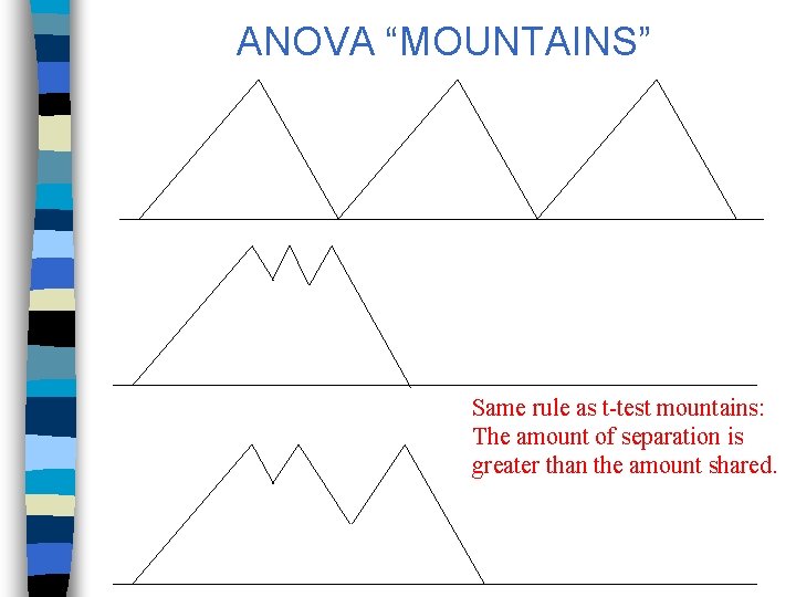
ANOVA “MOUNTAINS” Same rule as t-test mountains: The amount of separation is greater than the amount shared.

ANOVA TASK: Random Samples or Meaningfully Different Samples

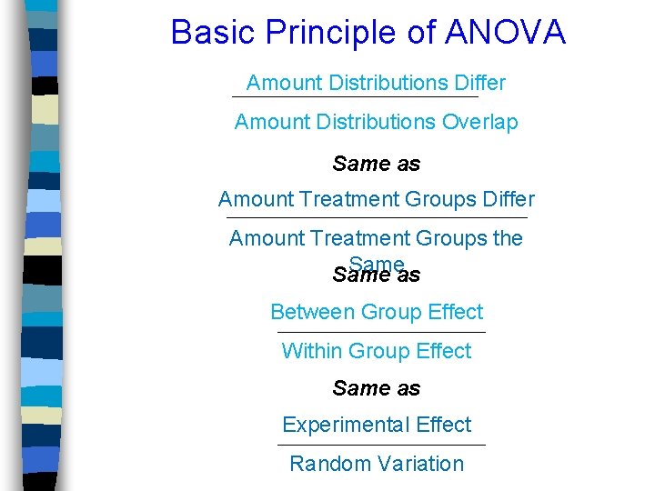
Basic Principle of ANOVA Amount Distributions Differ Amount Distributions Overlap Same as Amount Treatment Groups Differ Amount Treatment Groups the Sameas Same Between Group Effect Within Group Effect Same as Experimental Effect Random Variation

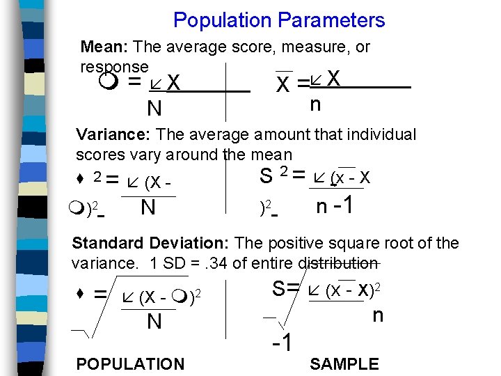
Population Parameters Mean: The average score, measure, or response = X = X n N Variance: The average amount that individual scores vary around the mean 2 = (x - X 2 S = (X - )2 )2 N n -1 Standard Deviation: The positive square root of the variance. 1 SD =. 34 of entire distribution = (X - N POPULATION )2 S= (x - X)2 n -1 SAMPLE

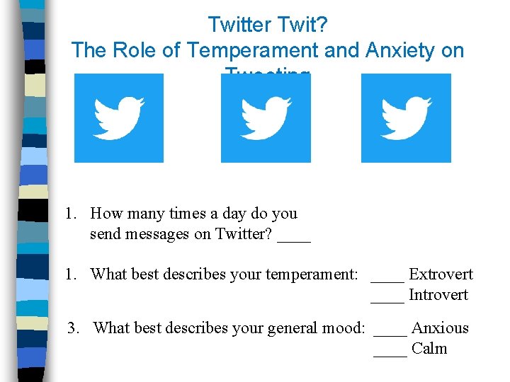
Twitter Twit? The Role of Temperament and Anxiety on Tweeting 1. How many times a day do you send messages on Twitter? ____ 1. What best describes your temperament: ____ Extrovert ____ Introvert 3. What best describes your general mood: ____ Anxious ____ Calm

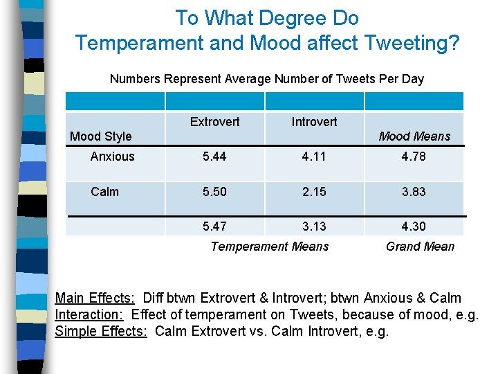
To What Degree Do Temperament and Mood affect Tweeting? Numbers Represent Average Number of Tweets Per Day Extrovert Introvert Mood Style Mood Means Anxious 5. 44 4. 11 4. 78 Calm 5. 50 2. 15 3. 83 5. 47 3. 13 4. 30 Temperament Means Grand Mean Main Effects: Diff btwn Extrovert & Introvert; btwn Anxious & Calm Interaction: Effect of temperament on Tweets, because of mood, e. g. Simple Effects: Calm Extrovert vs. Calm Introvert, e. g.

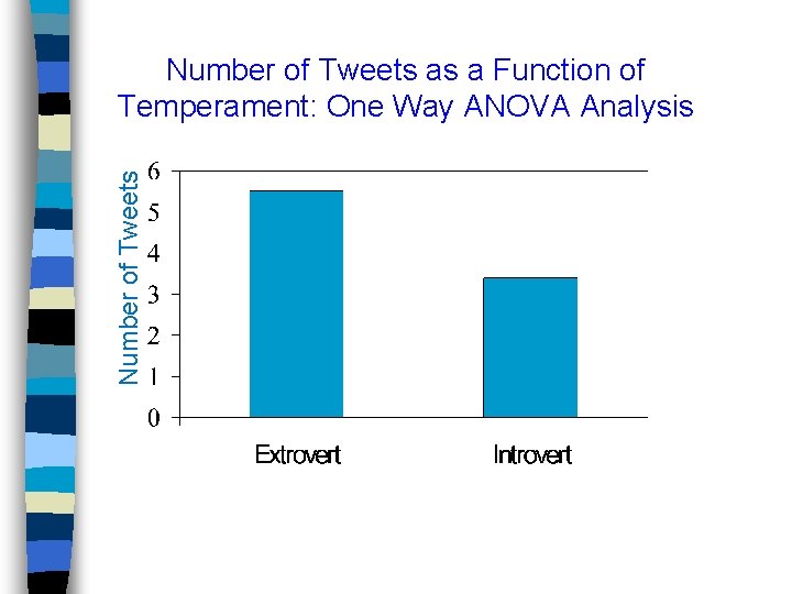
Number of Tweets as a Function of Temperament: One Way ANOVA Analysis

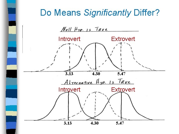
Do Means Significantly Differ? Introvert 3. 13 Extrovert 4. 30 Introvert 3. 13 5. 47 Extrovert 4. 30 5. 47

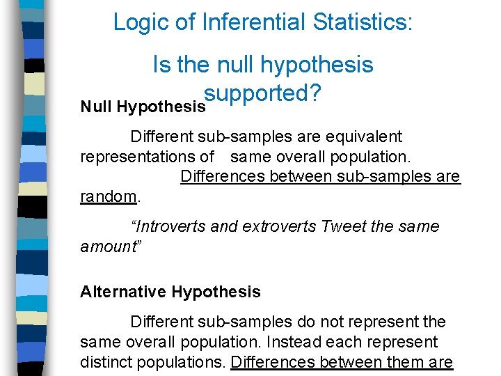
Logic of Inferential Statistics: Is the null hypothesis supported? Null Hypothesis Different sub-samples are equivalent representations of same overall population. Differences between sub-samples are random. “Introverts and extroverts Tweet the same amount” Alternative Hypothesis Different sub-samples do not represent the same overall population. Instead each represent distinct populations. Differences between them are

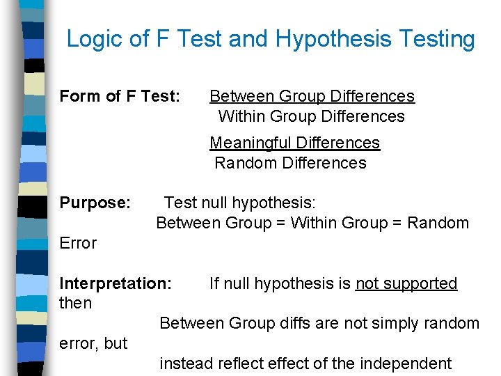
Logic of F Test and Hypothesis Testing Form of F Test: Between Group Differences Within Group Differences Meaningful Differences Random Differences Purpose: Test null hypothesis: Between Group = Within Group = Random Error Interpretation: If null hypothesis is not supported then Between Group diffs are not simply random error, but instead reflect effect of the independent

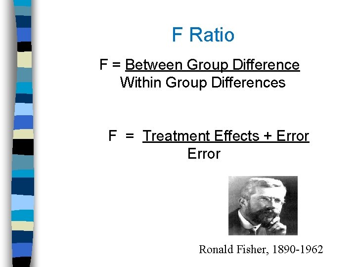
F Ratio F = Between Group Difference Within Group Differences F = Treatment Effects + Error Error Ronald Fisher, 1890 -1962

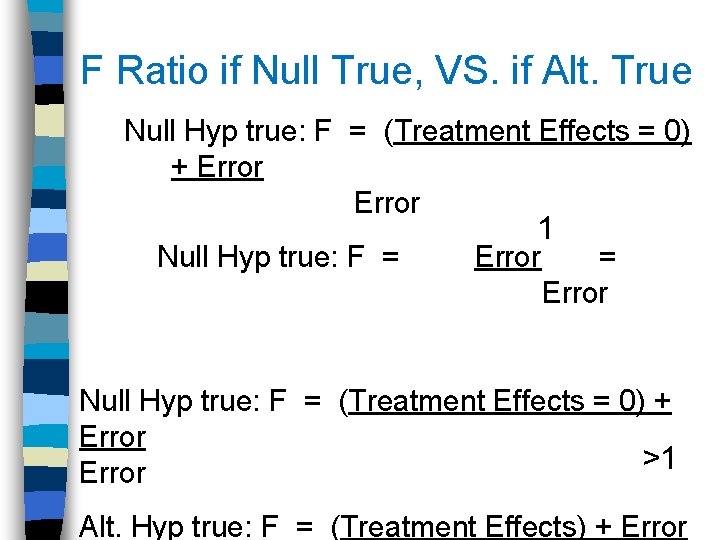
F Ratio if Null True, VS. if Alt. True Null Hyp true: F = (Treatment Effects = 0) + Error Error 1 Null Hyp true: F = Error = Error Null Hyp true: F = (Treatment Effects = 0) + Error >1 Error Alt. Hyp true: F = (Treatment Effects) + Error

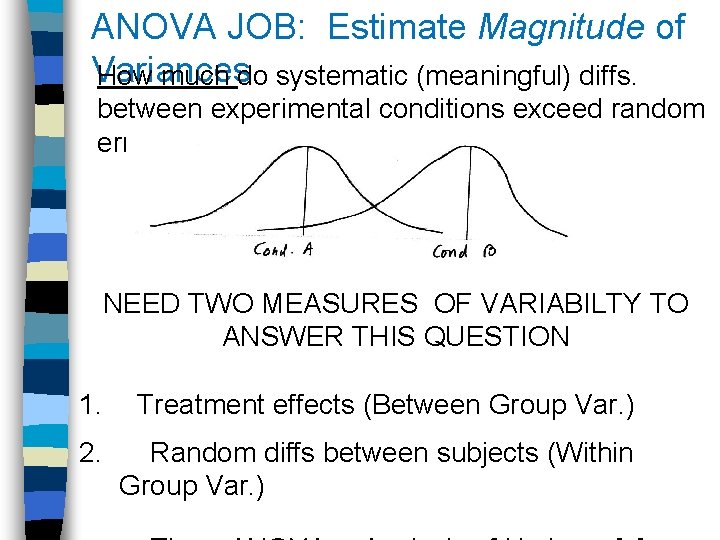
ANOVA JOB: Estimate Magnitude of Variances How much do systematic (meaningful) diffs. between experimental conditions exceed random error? NEED TWO MEASURES OF VARIABILTY TO ANSWER THIS QUESTION 1. Treatment effects (Between Group Var. ) 2. Random diffs between subjects (Within Group Var. )

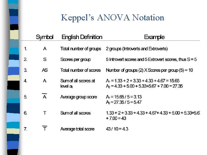
Keppel’s ANOVA Notation

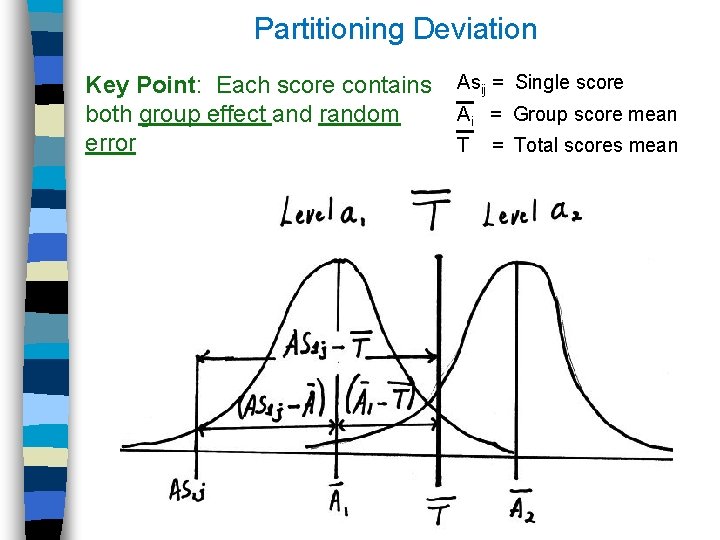
Partitioning Deviation Key Point: Each score contains Asij = Single score Ai = Group score mean both group effect and random error T = Total scores mean

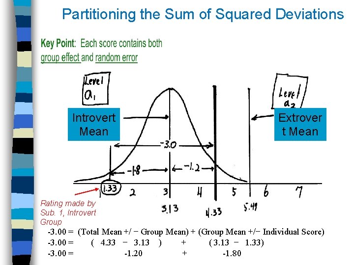
Partitioning the Sum of Squared Deviations Introvert Mean Extrover t Mean Rating made by Sub. 1, Introvert Group -3. 00 = (Total Mean +/ − Group Mean) + (Group Mean +/− Individual Score) -3. 00 = ( 4. 33 − 3. 13 ) + ( 3. 13 − 1. 33) -3. 00 = -1. 20 + -1. 80

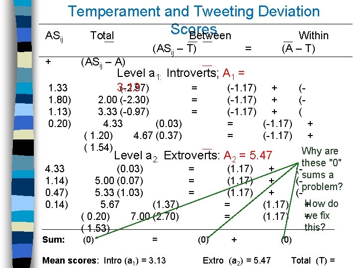
ASij + Temperament and Tweeting Deviation Scores Total Between Within (ASij – A) (ASij – T) = (A – T) Level a 1: Introverts; A 1 = 3. 13 (-2. 97) = (-1. 17) + 1. 33 1. 80) 2. 00 (-2. 30) = 1. 13) 3. 33 (-0. 97) = 0. 20) 4. 33 (0. 03) ( 1. 20) 4. 67 (0. 37) ( 1. 54) ((-1. 17) + ((-1. 17) + ( = (-1. 17) + Why are these "0" (1. 17) + (sums a (1. 17) + (problem? (1. 17) + (How do = (1. 17) + we fix = (1. 17) + this? Level a 2: Extroverts: A 2 = 5. 47 4. 33 (0. 03) = 1. 14) 5. 00 (0. 07) = 0. 47) 5. 33 (1. 03) = 0. 14) 5. 67 (1. 37) ( 0. 20) 7. 00 (2. 70) ( 1. 53) Sum: (0) = Mean scores: Intro (a 1) = 3. 13 (0) + (0) Extro (a 2) = 5. 47 Total (T) =

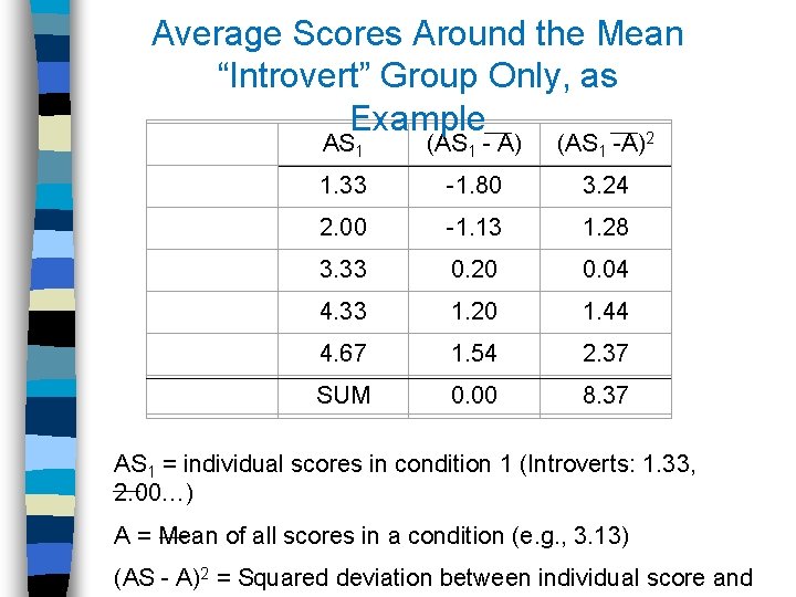
Average Scores Around the Mean “Introvert” Group Only, as Example 2 AS 1 (AS 1 - A) (AS 1 -A) 1. 33 -1. 80 3. 24 2. 00 -1. 13 1. 28 3. 33 0. 20 0. 04 4. 33 1. 20 1. 44 4. 67 1. 54 2. 37 SUM 0. 00 8. 37 AS 1 = individual scores in condition 1 (Introverts: 1. 33, 2. 00…) A = Mean of all scores in a condition (e. g. , 3. 13) (AS - A)2 = Squared deviation between individual score and

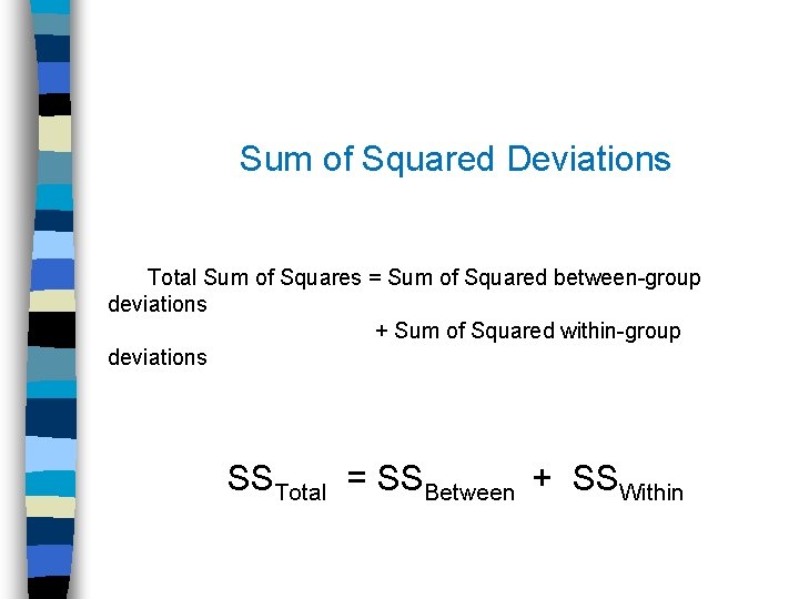
Sum of Squared Deviations Total Sum of Squares = Sum of Squared between-group deviations + Sum of Squared within-group deviations SSTotal = SSBetween + SSWithin

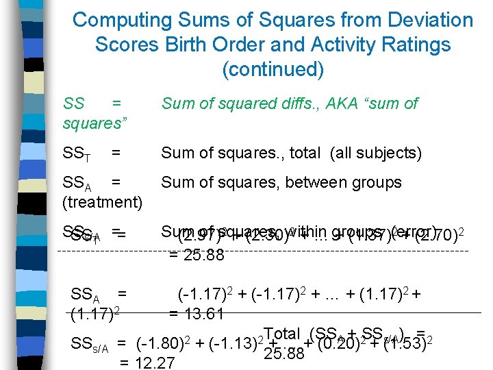
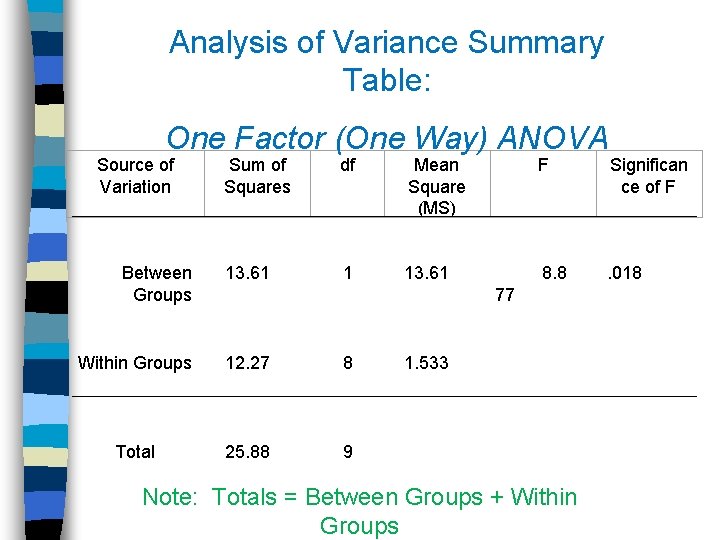
Computing Sums of Squares from Deviation Scores Birth Order and Activity Ratings (continued) SS = squares” Sum of squared diffs. , AKA “sum of SST Sum of squares. , total (all subjects) = SSA = (treatment) Sum of squares, between groups SS = SSs/AT = Sum of squares, within groups (error) (2. 97)2 + (2. 30)2 + … + (1. 37)2 + (2. 70)2 = 25. 88 SSA = (1. 17)2 (-1. 17)2 + … + (1. 17)2 + = 13. 61 Total (SSA + SS s/A) = 2 2 2 SSs/A = (-1. 80) + (-1. 13) + … + (0. 20) + (1. 53)2 25. 88 = 12. 27

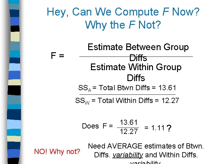
Hey, Can We Compute F Now? Why the F Not? Estimate Between Group Diffs Estimate Within Group Diffs F = SSA = Total Btwn Diffs = 13. 61 SSW = Total Within Diffs = 12. 27 Does F = 13. 61 = 1. 11 ? 12. 27 NO! Why not? Need AVERAGE estimates of Btwn. Diffs. variability and Within Diffs.

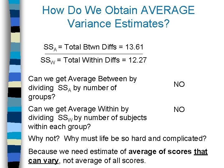
How Do We Obtain AVERAGE Variance Estimates? SSA = Total Btwn Diffs = 13. 61 SSW = Total Within Diffs = 12. 27 Can we get Average Between by dividing SSA by number of groups? Can we get Average Within by dividing SSW by number of subjects within each group? NO NO Why not? Why must life be so hard and complicated? Because we need estimate of average of scores that can vary, not average of all scores.

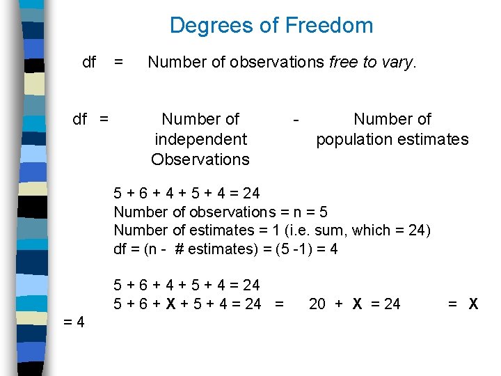
Degrees of Freedom df = Number of observations free to vary. df = Number of independent Observations - Number of population estimates 5 + 6 + 4 + 5 + 4 = 24 Number of observations = n = 5 Number of estimates = 1 (i. e. sum, which = 24) df = (n - # estimates) = (5 -1) = 4 5 + 6 + 4 + 5 + 4 = 24 5 + 6 + X + 5 + 4 = 24 = 20 + X = 24 = X = 4

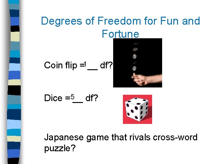
Degrees of Freedom for Fun and Fortune 1 Coin flip = __ df? 5 Dice = __ df? Japanese game that rivals cross-word puzzle?

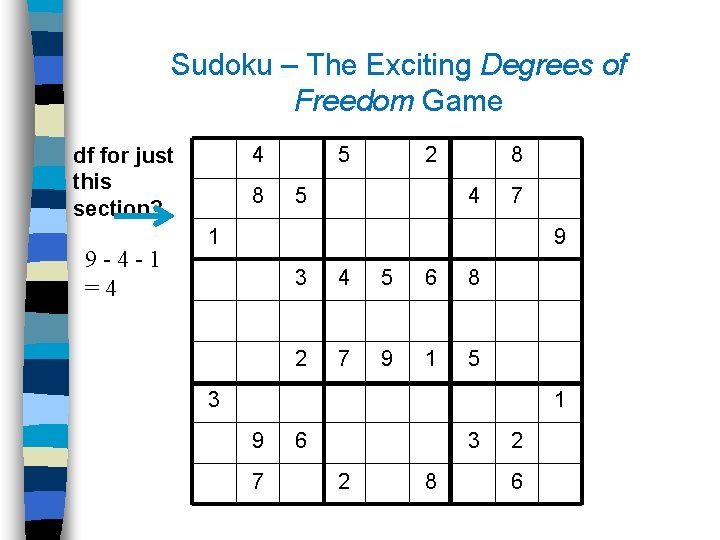
Sudoku – The Exciting Degrees of Freedom Game 4 df for just this section? 9 -4 -1 =4 8 5 2 5 8 4 7 1 9 3 4 5 6 8 2 7 9 1 5 3 1 9 7 6 3 2 8 2 6

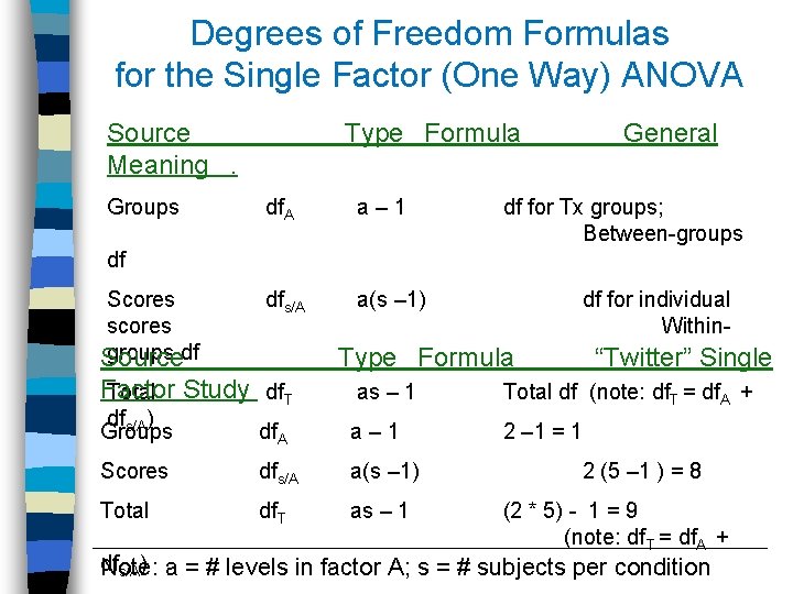
Degrees of Freedom Formulas for the Single Factor (One Way) ANOVA Source Meaning . Groups Type Formula General df. A a – 1 dfs/A a(s – 1) df for Tx groups; Between-groups df Scores scores groups df Source Type Formula “Twitter” Single Factor Study Total df. T as – 1 dfs/A) Groups df. A a – 1 Scores dfs/A a(s – 1) Total df for individual Within. Total df (note: df. T = df. A + 2 – 1 = 1 2 (5 – 1 ) = 8 df. T (2 * 5) - 1 = 9 as – 1 (note: df T = df. A + df Note: a = # levels in factor A; s = # subjects per condition s/A)

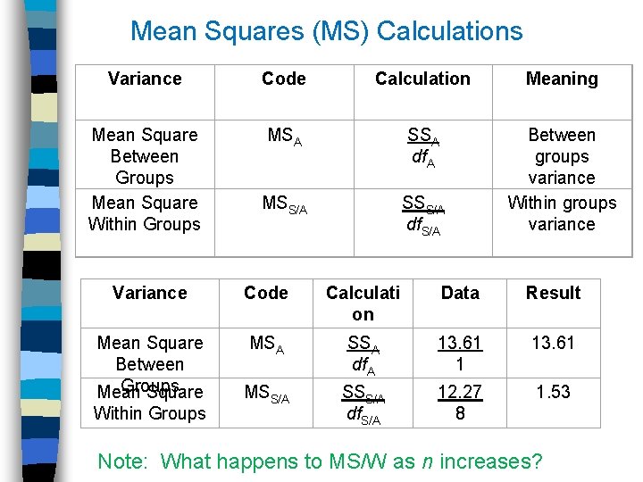
Mean Squares (MS) Calculations Variance Code Calculation Meaning Mean Square Between Groups Mean Square Within Groups MSA SSA df. A MSS/A SSS/A df. S/A Between groups variance Within groups variance Variance Code Calculati on Data Result Mean Square Between Groups Mean Square MSA SSA df. A 13. 61 1 13. 61 MSS/A SSS/A df. S/A 12. 27 8 1. 53 Within Groups Note: What happens to MS/W as n increases?

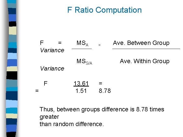
F Ratio Computation F = Variance MSA = Ave. Between Group Variance MSS/A Ave. Within Group F = 13. 61 1. 51 = 8. 78 Thus, between groups difference is 8. 78 times greater than random difference.

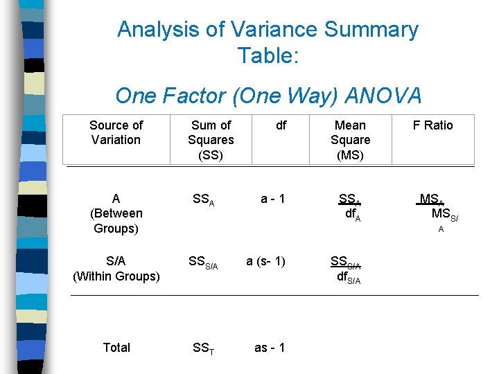
Analysis of Variance Summary Table: One Factor (One Way) ANOVA Source of Variation A (Between Groups) Sum of Squares (SS) SSA S/A SSS/A (Within Groups) Total df Mean Square (MS) a - 1 F Ratio SSA df. A a (s- 1) MSA MSS/ SSS/A df. S/A SST as - 1 A

Analysis of Variance Summary Table: One Factor (One Way) ANOVA Source of Variation Sum of Squares Between Groups df 13. 61 Within Groups 12. 27 Total 25. 88 Mean Square (MS) 1 8 9 13. 61 F 8. 8 77 . 018 1. 533 Note: Totals = Between Groups + Within Groups Significan ce of F

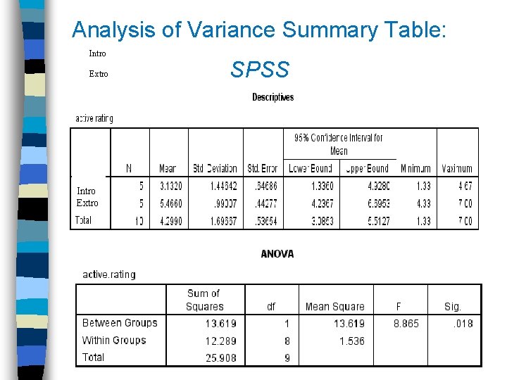
Analysis of Variance Summary Table: Intro Extro SPSS

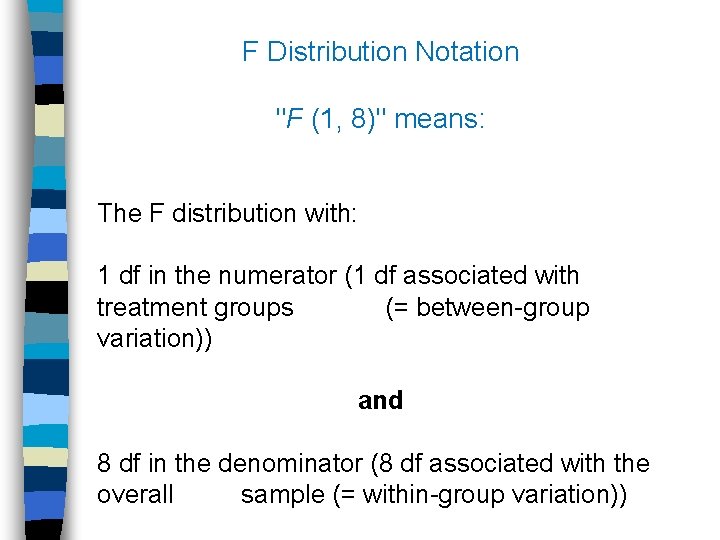
F Distribution Notation "F (1, 8)" means: The F distribution with: 1 df in the numerator (1 df associated with treatment groups (= between-group variation)) and 8 df in the denominator (8 df associated with the overall sample (= within-group variation))

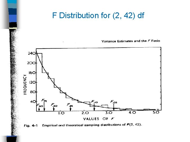
F Distribution for (2, 42) df

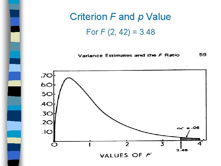
Criterion F and p Value For F (2, 42) = 3. 48

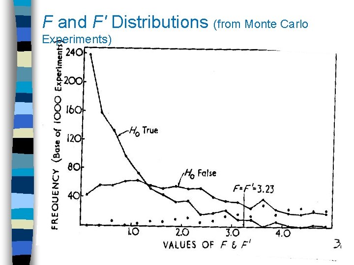
F and F' Distributions (from Monte Carlo Experiments)

Which Distribution Do Data Support: F or F′? If F is correct, then Ho supported: u 1 = u 2 (Introvert = Extrovert) If F' is correct, then H 1 supported: u 1 u 2 (Introvert ≠ Extrovert)

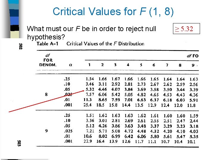
Critical Values for F (1, 8) What must our F be in order to reject null hypothesis? ≥ 5. 32

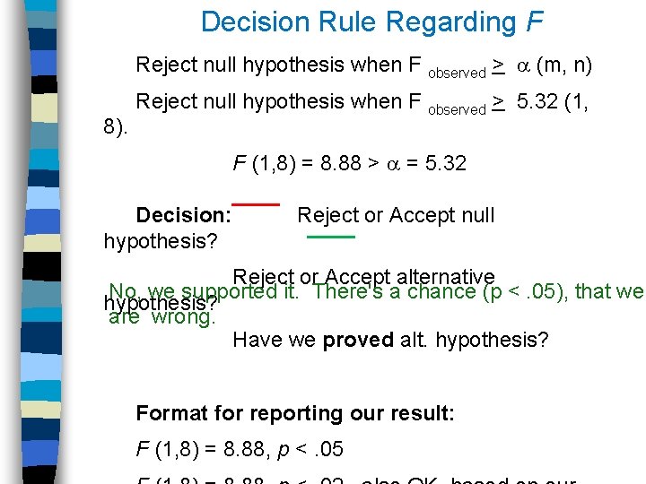
Decision Rule Regarding F Reject null hypothesis when F observed > (m, n) 8). Reject null hypothesis when F observed > 5. 32 (1, F (1, 8) = 8. 88 > = 5. 32 Decision: hypothesis? Reject or Accept null Reject or Accept alternative No, we supported it. There's a chance (p <. 05), that we hypothesis? are wrong. Have we proved alt. hypothesis? Format for reporting our result: F (1, 8) = 8. 88, p <. 05

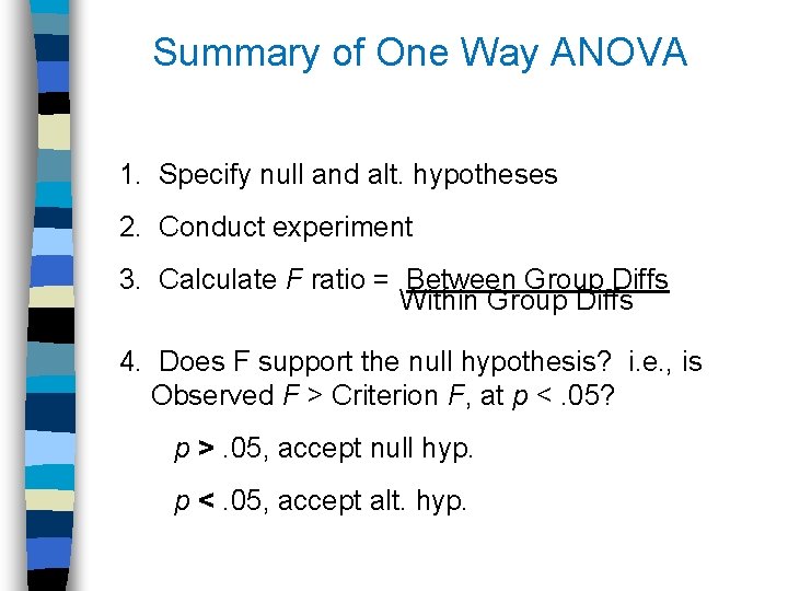
Summary of One Way ANOVA 1. Specify null and alt. hypotheses 2. Conduct experiment 3. Calculate F ratio = Between Group Diffs Within Group Diffs 4. Does F support the null hypothesis? i. e. , is Observed F > Criterion F, at p <. 05? p >. 05, accept null hyp. p <. 05, accept alt. hyp.

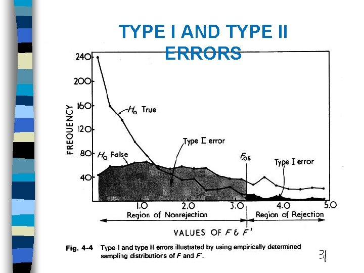
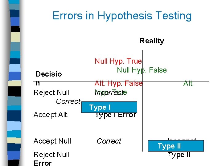
TYPE I AND TYPE II ERRORS

Errors in Hypothesis Testing Reality Null Hyp. True Null Hyp. False Decisio n Alt. Hyp. False Hyp. True Reject Null Incorrect: Correct Type I Accept Alt. Type Error I Error Accept Null Correct Reject Null Error Alt. Incorrect: Type II Type Error II

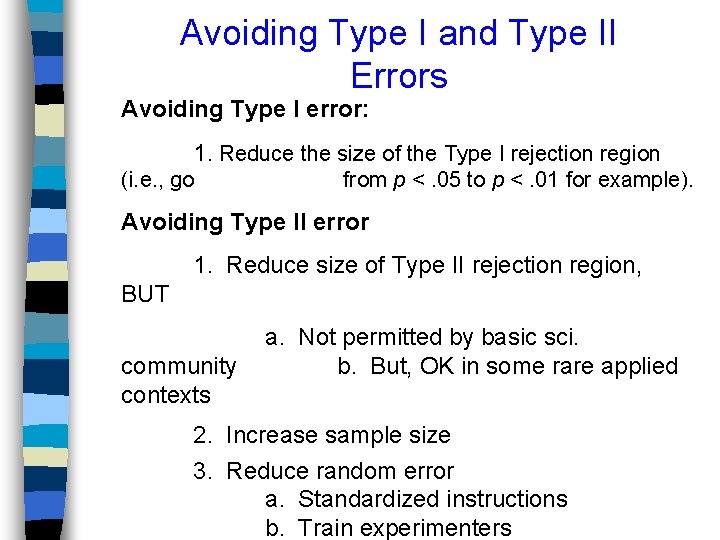
Avoiding Type I and Type II Errors Avoiding Type I error: 1. Reduce the size of the Type I rejection region (i. e. , go from p <. 05 to p <. 01 for example). Avoiding Type II error 1. Reduce size of Type II rejection region, BUT community contexts a. Not permitted by basic sci. b. But, OK in some rare applied 2. Increase sample size 3. Reduce random error a. Standardized instructions b. Train experimenters