Nonlinear Spectral Analysis in Aeroacoustics Dr K Srinivasan

Nonlinear Spectral Analysis in Aeroacoustics Dr. K. Srinivasan Department of Mechanical Engineering Indian Institute of Technology Madras

Acknowledgement • Funding agencies: – AFOSR (Dr. John Schmisseur) – ISRO (ISRO-IITM Cell) • Co-researchers: – – – – – Prof. Ganesh Raman, IIT, Chicago Prof. David Williams, IIT Chicago Prof. K. Ramamurthi, IIT Madras Prof. T. Sundararajan, IIT Madras Dr. Byung Hun-Kim, IIT, Chicago Dr. Praveen Panickar, IIT, Chicago Mr. Rahul Joshi, IIT Chicago Mr. S. Narayanan, IIT Madras Mr. P. Bhave, IIT Madras 2

Roadmap of the talk • Examples of nonlinearity in aeroacoustics – Twin jet coupling – Hartmann whistle • Twin jet coupling: Results from linear spectral analysis • Motivation to use nonlinear spectral analysis • Results from nonlinear spectra • Interaction density metric • Universality of interaction density metric • Conclusions 3

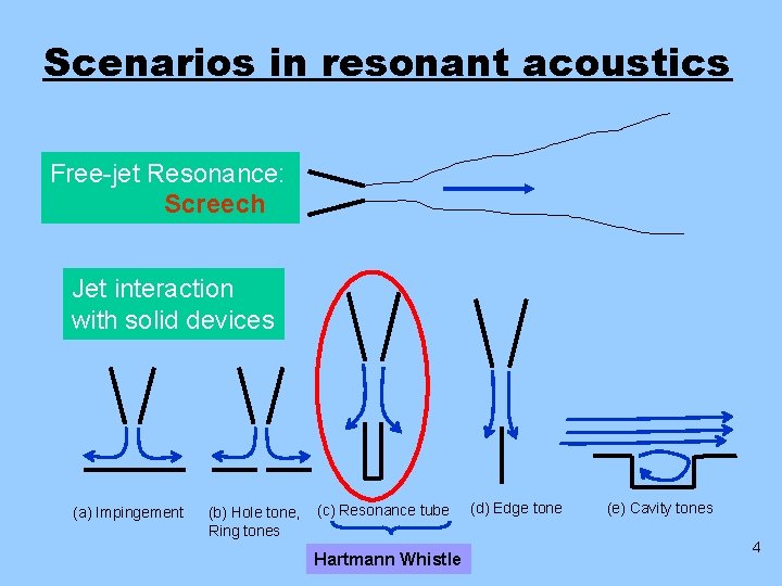
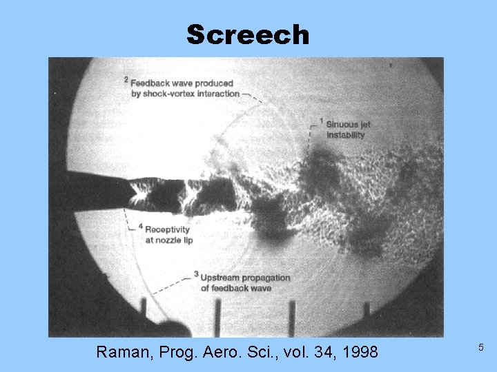
Scenarios in resonant acoustics Free-jet Resonance: Screech Jet interaction with solid devices (a) Impingement (b) Hole tone, Ring tones (c) Resonance tube Hartmann Whistle (d) Edge tone (e) Cavity tones 4

Screech Raman, Prog. Aero. Sci. , vol. 34, 1998 5

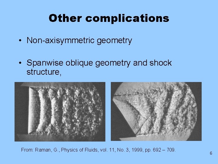
Other complications • Non-axisymmetric geometry • Spanwise oblique geometry and shock structure, From: Raman, G. , Physics of Fluids, vol. 11, No. 3, 1999, pp. 692 – 709. 6

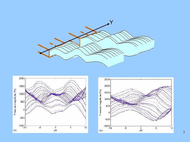
Y 7

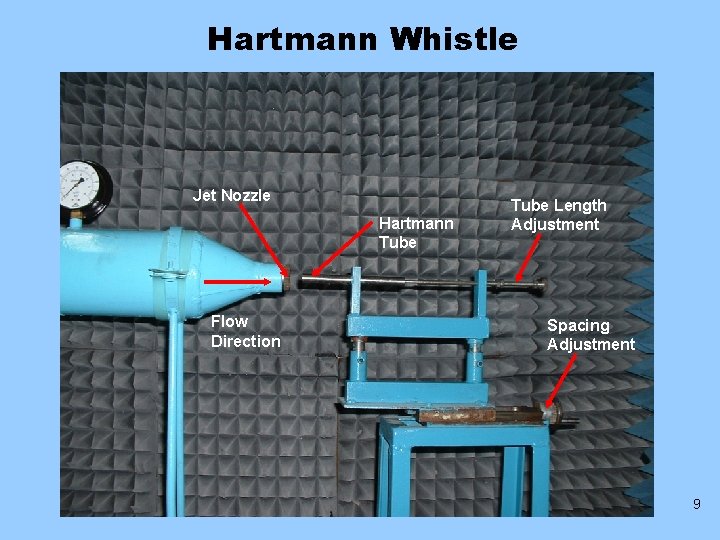
Hartmann Whistle

Hartmann Whistle Jet Nozzle Hartmann Tube Flow Direction Tube Length Adjustment Spacing Adjustment 9

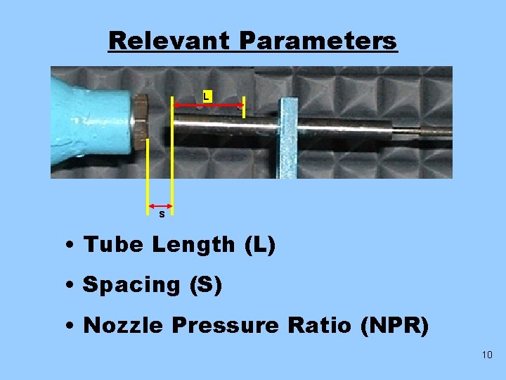
Relevant Parameters L s • Tube Length (L) • Spacing (S) • Nozzle Pressure Ratio (NPR) 10

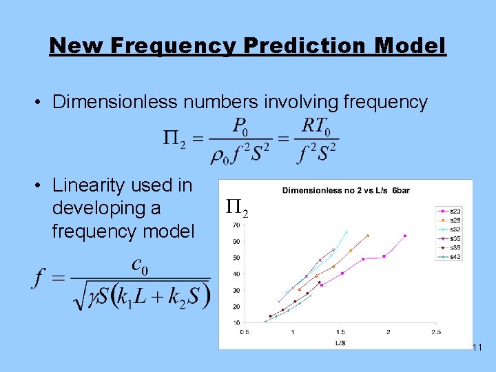
New Frequency Prediction Model • Dimensionless numbers involving frequency • Linearity used in developing a frequency model 11

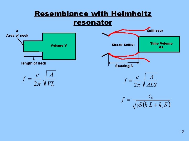
Resemblance with Helmholtz resonator Spill-over A Area of neck Volume V L length of neck Shock Cell(s) Tube Volume AL Spacing S 12

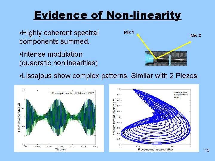
Evidence of Non-linearity • Highly coherent spectral components summed. Mic 1 Mic 2 • Intense modulation (quadratic nonlinearities) • Lissajous show complex patterns. Similar with 2 Piezos. 13

Twin jet Coupling

Literature on twin jet coupling • Berndt (1984) found enhanced dynamic pressure in a twin jet nacelle. • Tam, Seiner (1987) Twin plume screech. • Morris (1990) instability analysis of twin jet. • Wlezien (1987) Parameters influencing interactions. • Shaw (1990) Methods to suppress twinjet screech. • Raman, Taghavi (1996, 98) coupling modes, relation to shock cell spacing, etc. • Panickar, Srinivasan, and Raman (2004) Twin jets from two single beveled nozzles. • Joshi, Panickar, Srinivasan, and Raman (2006) Nozzle orientation effects and non-linearity 15

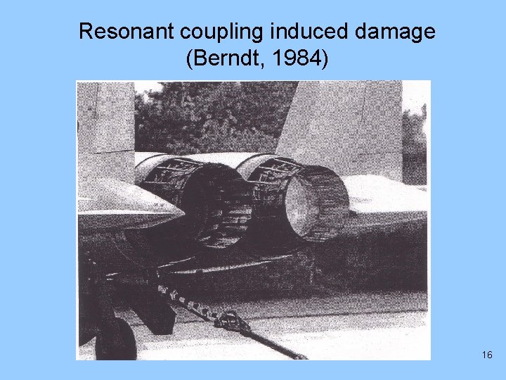
Resonant coupling induced damage (Berndt, 1984) 16

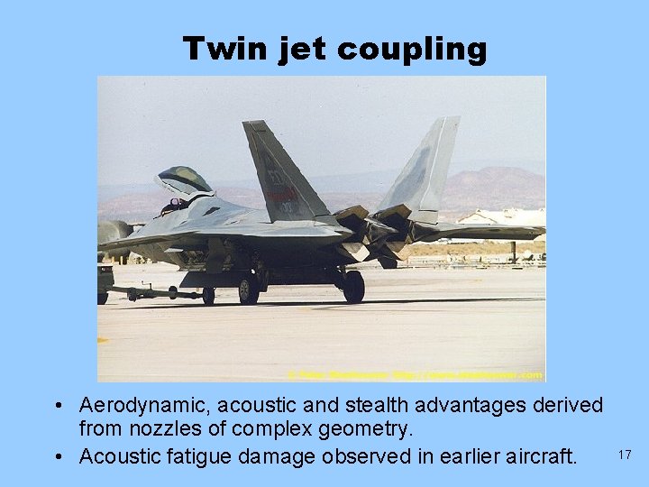
Twin jet coupling • Aerodynamic, acoustic and stealth advantages derived from nozzles of complex geometry. • Acoustic fatigue damage observed in earlier aircraft. 17

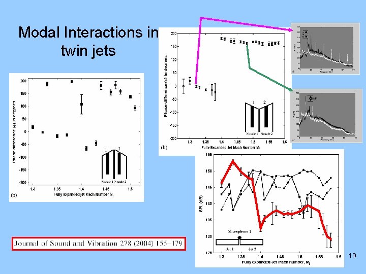
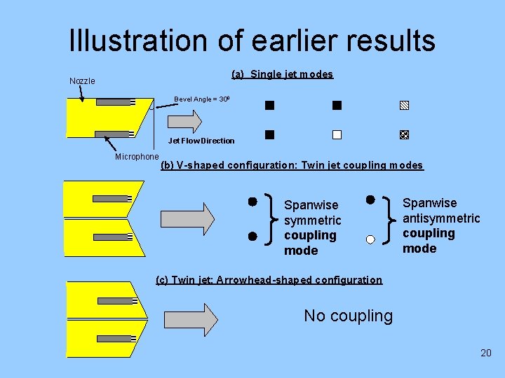
Our earlier work • Panickar et al. (2004) concluded the following from their experiments: – Single beveled jet - symm, antisymm and oblique modes. – Twin jet - only spanwise symmetric and antisymmetric modes during coupling. – A simple change to the configuration eliminated coupling between the jets. Journal of Sound and Vibration, vol. 278, pp. 155 -179, 2004. 18

Modal Interactions in twin jets 19

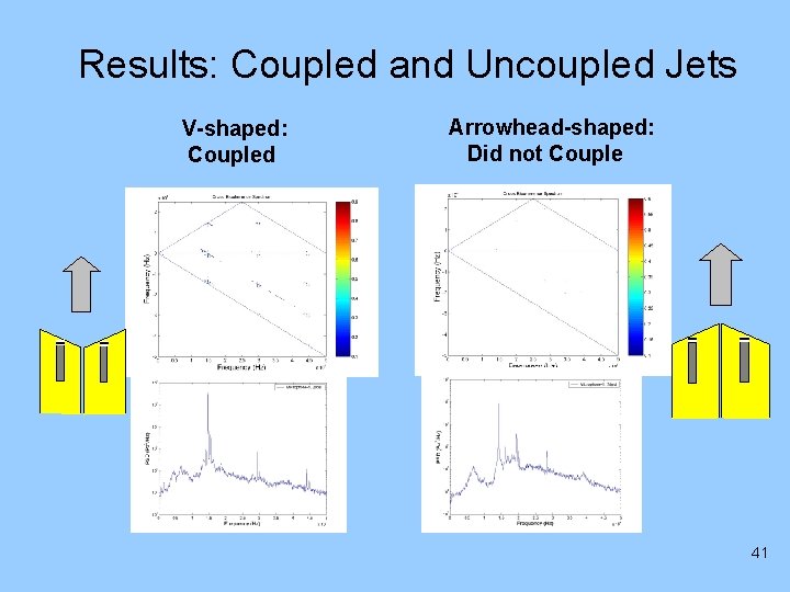
Illustration of earlier results (a) Single jet modes Nozzle Bevel Angle = 300 Jet Flow Direction Microphone (b) V-shaped configuration: Twin jet coupling modes Spanwise symmetric coupling mode Spanwise antisymmetric coupling mode (c) Twin jet: Arrowhead-shaped configuration No coupling 20

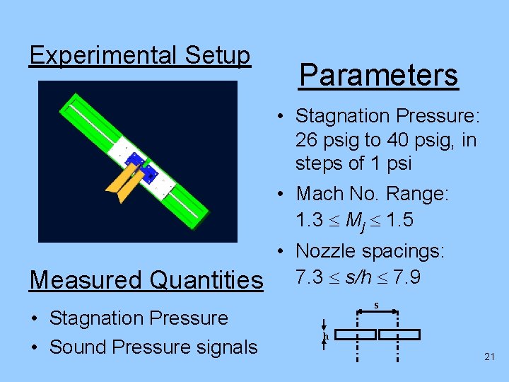
Experimental Setup Parameters • Stagnation Pressure: 26 psig to 40 psig, in steps of 1 psi • Mach No. Range: 1. 3 Mj 1. 5 Measured Quantities • Stagnation Pressure • Sound Pressure signals • Nozzle spacings: 7. 3 s/h 7. 9 s h 21

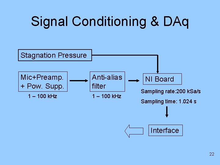
Signal Conditioning & DAq Stagnation Pressure Mic+Preamp. + Pow. Supp. Anti-alias filter 1 – 100 k. Hz NI Board Sampling rate: 200 k. Sa/s Sampling time: 1. 024 s Interface 22

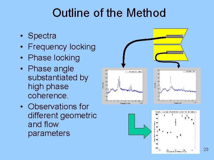
Outline of the Method • • Spectra Frequency locking Phase angle substantiated by high phase coherence. • Observations for different geometric and flow parameters 23

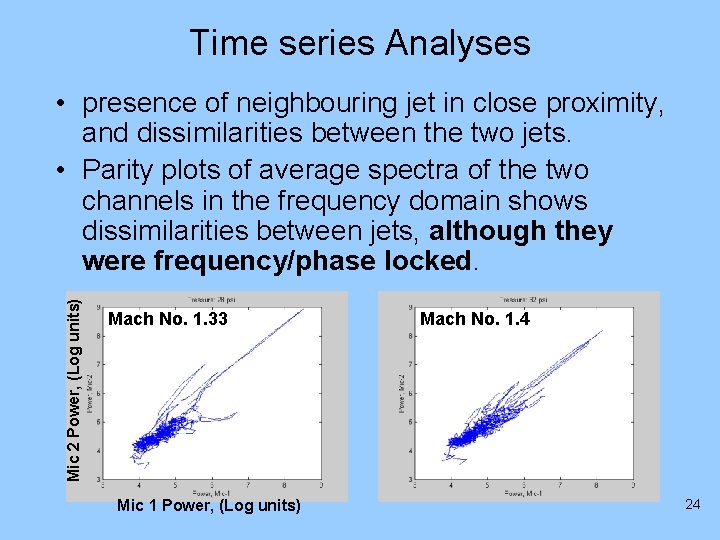
Time series Analyses Mic 2 Power, (Log units) • presence of neighbouring jet in close proximity, and dissimilarities between the two jets. • Parity plots of average spectra of the two channels in the frequency domain shows dissimilarities between jets, although they were frequency/phase locked. Mach No. 1. 33 Mic 1 Power, (Log units) Mach No. 1. 4 24

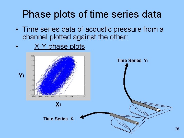
Phase plots of time series data • Time series data of acoustic pressure from a channel plotted against the other: • X-Y phase plots Time Series: Yi Yi Xi Time Series: Xi 25

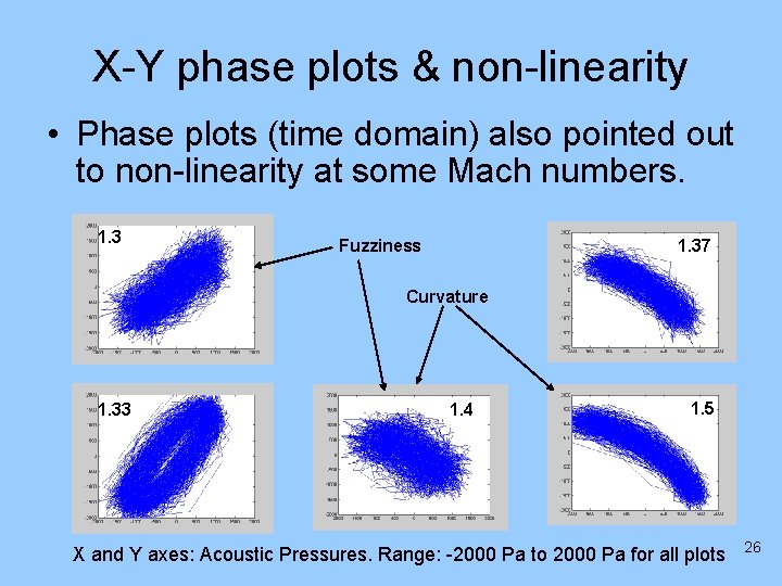
X-Y phase plots & non-linearity • Phase plots (time domain) also pointed out to non-linearity at some Mach numbers. 1. 3 Fuzziness 1. 37 Curvature 1. 33 1. 4 1. 5 X and Y axes: Acoustic Pressures. Range: -2000 Pa to 2000 Pa for all plots 26

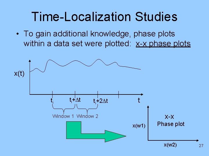
Time-Localization Studies • To gain additional knowledge, phase plots within a data set were plotted: x-x phase plots x(t) ti ti+ t ti+2 t t x-x Window 1 Window 2 x(w 1) Phase plot x(w 2) 27

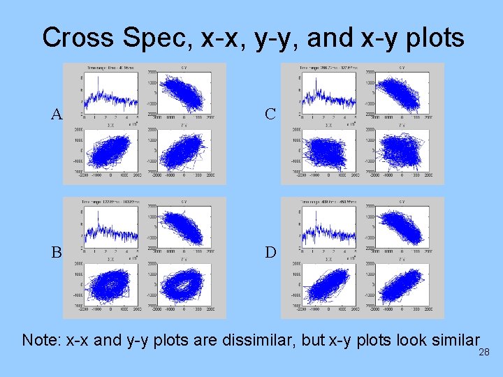
Cross Spec, x-x, y-y, and x-y plots A C B D Note: x-x and y-y plots are dissimilar, but x-y plots look similar 28

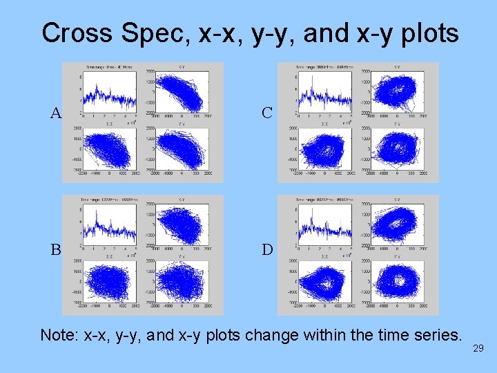
Cross Spec, x-x, y-y, and x-y plots A C B D Note: x-x, y-y, and x-y plots change within the time series. 29

Further attempts to understand the -linear behaviour non • Simulation of non-linear sinusoids to match their phase plots with experimental ones. – A Lissajou simulator for generating various artificial phase plots. – These attempts were not much successful and not an elegant approach to decipher the non-linearities. • Conventional spectral analysis (SOS) does not reveal information about nonlinearities. 30

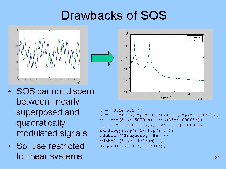
Drawbacks of SOS • SOS cannot discern between linearly superposed and quadratically modulated signals. • So, use restricted to linear systems. t = [0: 1 e-5: 1]'; x = 0. 5*(sin(2*pi*3000*t)+sin(2*pi*13000*t)); y = sin(2*pi*5000*t). *sin(2*pi*8000*t); [p f] = spectrum(x, y, 1024, [], 100000); semilogy(f, p(: , 1), f, p(: , 2)); xlabel ('Frequency (Hz)'); ylabel ('PSD (1^2/Hz)'); legend('3 k+13 k', '5 k*8 k'); 31

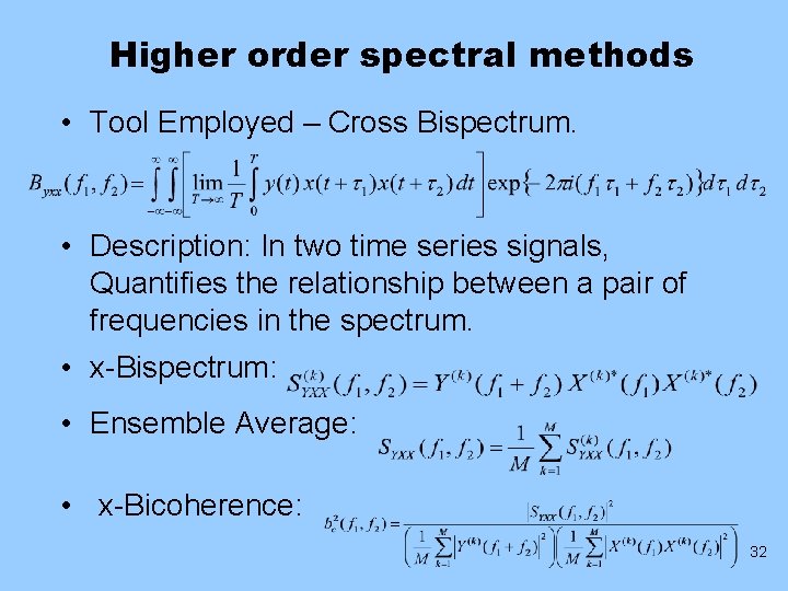
Higher order spectral methods • Tool Employed – Cross Bispectrum. • Description: In two time series signals, Quantifies the relationship between a pair of frequencies in the spectrum. • x-Bispectrum: • Ensemble Average: • x-Bicoherence: 32

Use of HOS in shear flows • Thomas and Chu (1991, 1993): Planar shear layers, traced the axial evolution of modes. • Walker & Thomas (1997): Screeching rectangular jet, axial evolution of nonlinear interactions. • Thomas (2003): Book chapter on HOS tools applicable to shear flows. 33

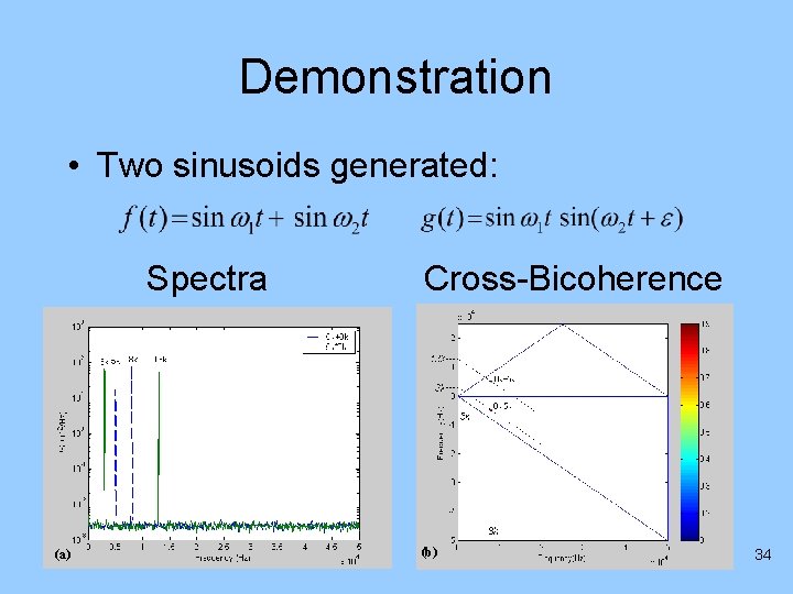
Demonstration • Two sinusoids generated: Spectra (a) Cross-Bicoherence (b) 34

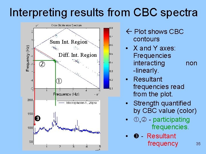
Interpreting results from CBC spectra Sum Int. Region Diff. Int. Region Plot shows CBC contours • X and Y axes: Frequencies interacting non -linearly. • Resultant frequencies read from the plot. • Strength quantified by CBC value (color) • , - participating frequencies. • - Resultant 35 frequency

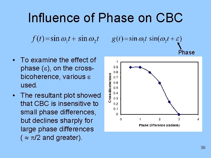
Influence of Phase on CBC Phase • To examine the effect of phase ( ), on the crossbicoherence, various used. • The resultant plot showed that CBC is insensitive to small phase differences, but declines sharply for large phase differences ( /2 and greater). 36

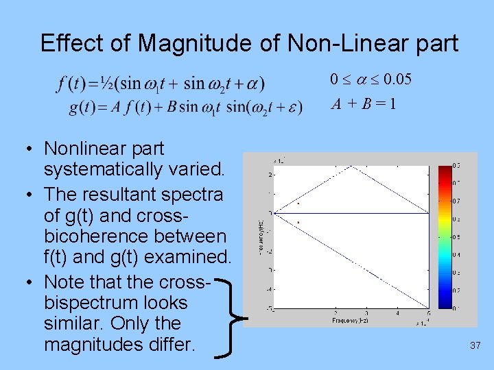
Effect of Magnitude of Non-Linear part 0 0. 05 A + B = 1 • Nonlinear part systematically varied. • The resultant spectra of g(t) and crossbicoherence between f(t) and g(t) examined. • Note that the crossbispectrum looks similar. Only the magnitudes differ. 37

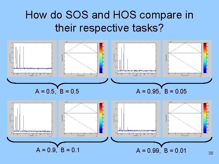
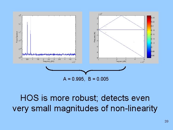
How do SOS and HOS compare in their respective tasks? A = 0. 5, B = 0. 5 A = 0. 95, B = 0. 05 A = 0. 9, B = 0. 1 A = 0. 99, B = 0. 01 38

A = 0. 995, B = 0. 005 HOS is more robust; detects even very small magnitudes of non-linearity 39

How to use CBC • Obtain the second order and third order spectra for the entire parametric space. • Look for changes in gross features in the higher order spectra and establish a correspondence with earlier knowledge. • Establish metrics from HOS to quantify non-linearity. • If possible, trace the evolution of the spectra. 40

Results: Coupled and Uncoupled Jets Arrowhead-shaped: Did not Couple V-shaped: Coupled 41

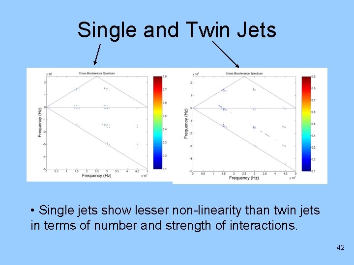
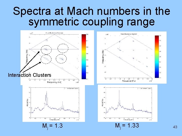
Single and Twin Jets • Single jets show lesser non-linearity than twin jets in terms of number and strength of interactions. 42

Spectra at Mach numbers in the symmetric coupling range Interaction Clusters Mj = 1. 33 43

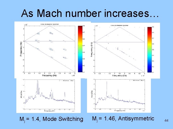
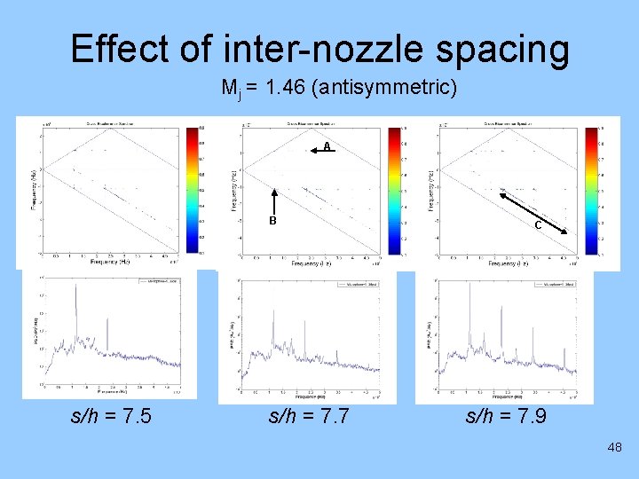
As Mach number increases… Mj = 1. 4, Mode Switching Mj = 1. 46, Antisymmetric 44

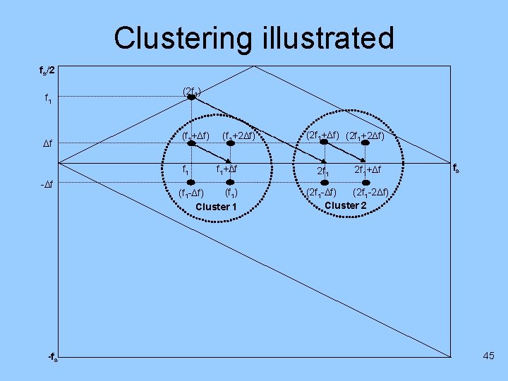
Clustering illustrated fs/2 f 1 f (2 f 1) (f 1+ f) f 1 - f -fs (f 1+2 f) f 1+ f (f 1) (f 1 - f) Cluster 1 (2 f 1+ f) (2 f 1+2 f) 2 f 1+ f fs (2 f 1 -2 f) (2 f 1 - f) Cluster 2 45

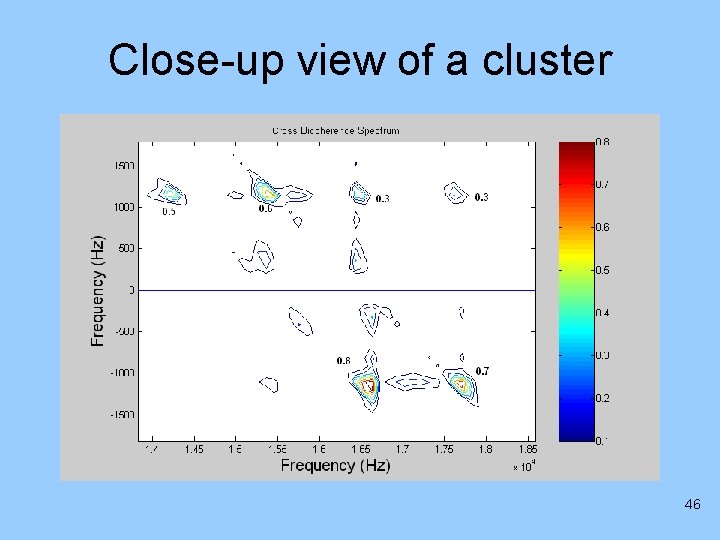
Close-up view of a cluster 46

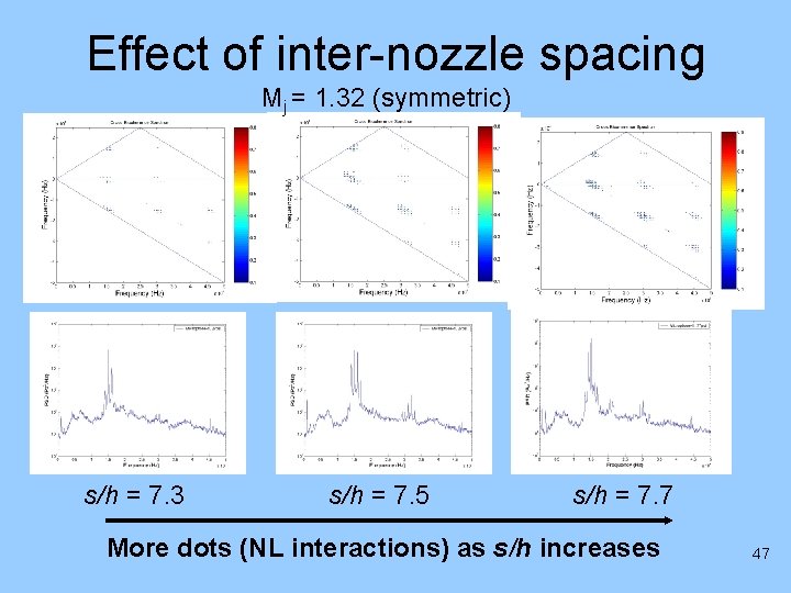
Effect of inter-nozzle spacing Mj = 1. 32 (symmetric) s/h = 7. 3 s/h = 7. 5 s/h = 7. 7 More dots (NL interactions) as s/h increases 47

Effect of inter-nozzle spacing Mj = 1. 46 (antisymmetric) A B s/h = 7. 5 s/h = 7. 7 C s/h = 7. 9 48

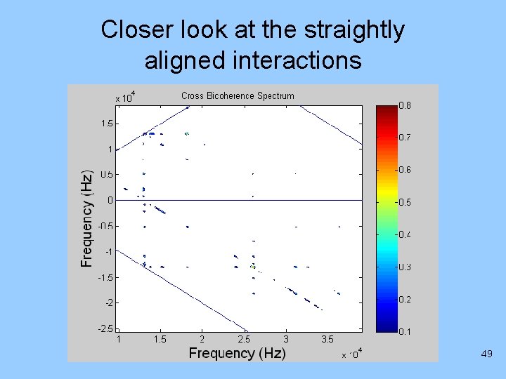
Closer look at the straightly aligned interactions 49

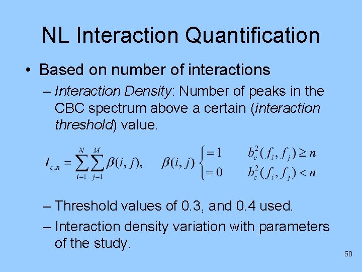
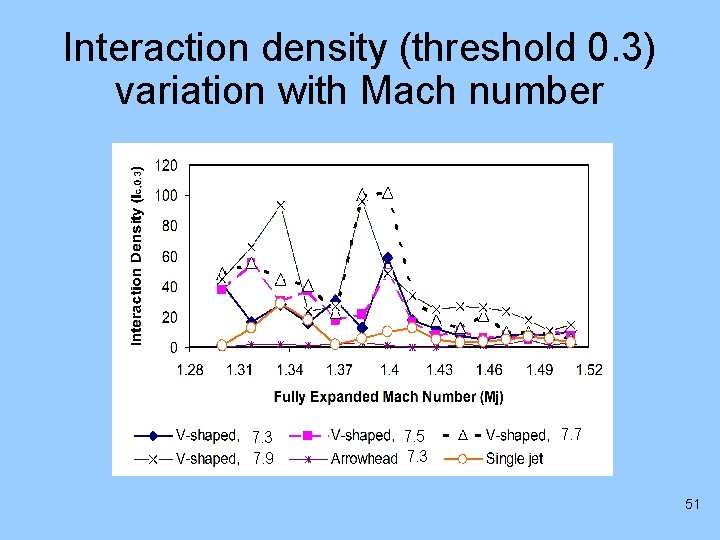
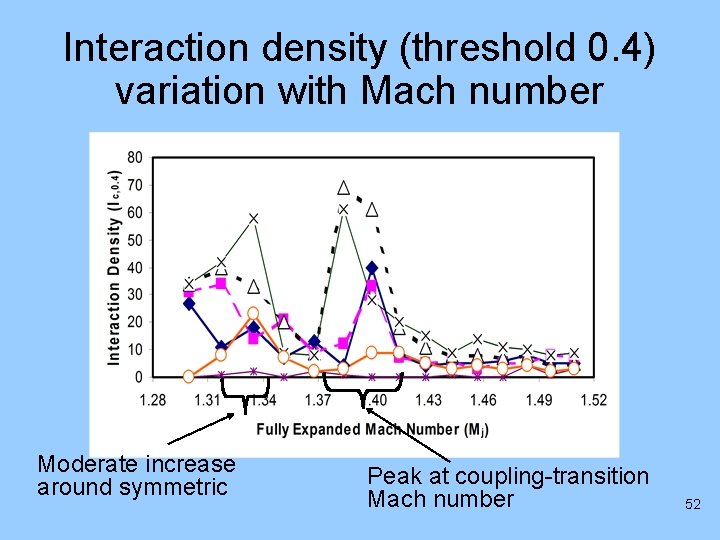
NL Interaction Quantification • Based on number of interactions – Interaction Density: Number of peaks in the CBC spectrum above a certain (interaction threshold) value. – Threshold values of 0. 3, and 0. 4 used. – Interaction density variation with parameters of the study. 50

Interaction density (threshold 0. 3) variation with Mach number 7. 3 7. 9 7. 5 7. 3 7. 7 51

Interaction density (threshold 0. 4) variation with Mach number Moderate increase around symmetric Peak at coupling-transition Mach number 52

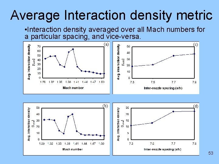
Average Interaction density metric • Interaction density averaged over all Mach numbers for a particular spacing, and vice-versa. (a) (c) (b) (d) 53

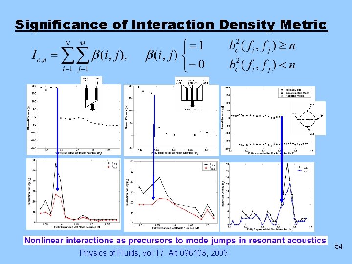
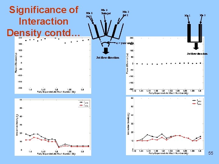
Significance of Interaction Density Metric Physics of Fluids, vol. 17, Art. 096103, 2005 54

Significance of Interaction Density contd… Mic 1 Jet 1 Mic 3 Twin jet Mic 2 Jet 2 Mic 1 Mic 2 α = yaw angle Jet flow direction 55

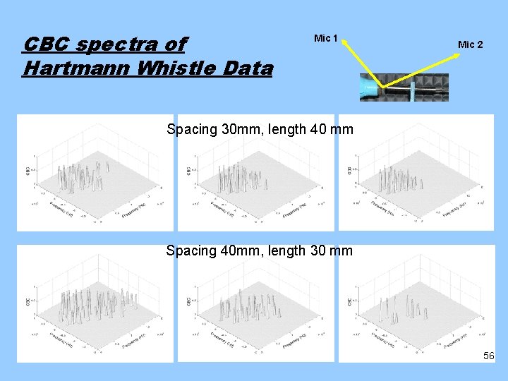
CBC spectra of Hartmann Whistle Data Mic 1 Mic 2 Spacing 30 mm, length 40 mm Spacing 40 mm, length 30 mm 56

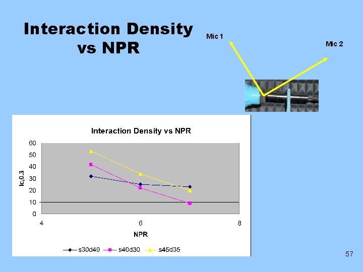
Interaction Density vs NPR Mic 1 Mic 2 57

Conclusions • Configurations that did not show conclusive linear coupling were found nonlinearly coupled. So, nonlinear coupling may be important in nozzle design. • Nonlinearity in configs can be graded • Two patterns of cross-bicoherence were observed, one that showed clustering, and another that showed a straight alignment. 58

Conclusions… • A new interaction density metric identified and seems a relevant parameter to quantify non-linear coupling. • The average interaction density peaks in the vicinity of mode jumps • Therefore, higher order spectra could serve as useful tools in theoretical understanding as well as in practical situations. 59

60