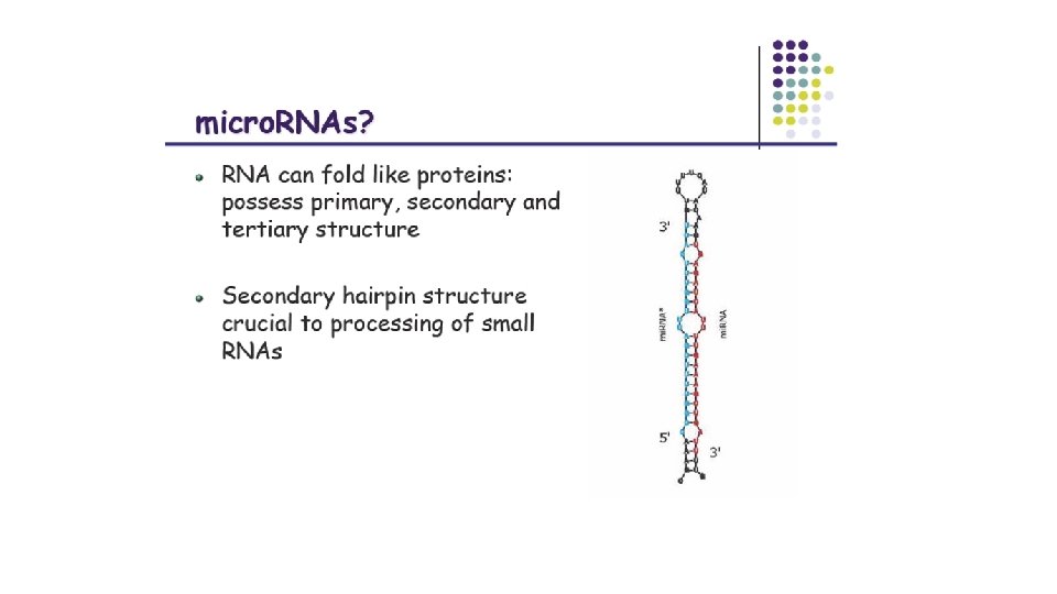
micro RNA computational prediction and analysis Resources Lecture

micro. RNA computational prediction and analysis

Resources • Lecture notes from previous years: Takis Benos and Ziv Bar-Joseph • Slides from: www. bioalgorithms. info

Discovery of small RNAs Rosalind Lee • The first small RNA: • In 1993 Rosalind Lee (Victor Ambros lab) was studying a noncoding gene in C. elegans, lin-4, that was involved in silencing of another gene, lin-14, at the appropriate time in the development of the worm C. elegans. • Two small transcripts of lin-4 (22 nt and 61 nt) were found to be complementary to a sequence in the 3' UTR of lin-14. • Because lin-4 encoded no protein, she deduced that it must be these transcripts that are causing the silencing by RNA-RNA interactions. • The second small RNA wasn't discovered until 2000!

What are small nc. RNAs? • Two flavors of small non-coding RNA: 1. micro RNA (mi. RNA) 2. short interfering RNA (si. RNA) • Properties of small non-coding RNA: • • Involved in silencing other m. RNA transcripts. Called “small” because they are usually only about 21 -24 nucleotides long. Synthesized by first cutting up longer precursor sequences (like the 61 nt one that Lee discovered). Silence an m. RNA by base pairing with some sequence on the m. RNA.

mi. RNA Pathway Illustration

si. RNA Pathway Illustration Complementary base pairing facilitates the m. RNA cleavage

Features of mi. RNAs • Hundreds mi. RNA genes are already identified in human genome. • Most mi. RNAs start with a U • The second 7 -mer on the 5' end is known as the “seed. ” • When an mi. RNAs bind to their targets, the seed sequence has perfect or nearperfect alignment to some part of the target sequence. • Example: UGAGCUUAGCAG. . .

Features of mi. RNAs • Many mi. RNAs are conserved across species: • For half of known human mi. RNAs, >18% of all occurrences of one of these mi. RNA seeds are conserved among human, dog, rat, and mouse. • As a rule, the full sequence of mi. RNAs is almost never completely complementary to the target sequence. • Common to see a loop or bulge after the seed when binding. • Loop/bulge is often a hairpin because of stability. • The site at which mi. RNAs attack is often in their target's 3' UTR.

mi. RNA Binding Bulges Hairpin is more stable than a simple bulge The MRE is known as the “mi. RNA recognition element. ” This is simply the sequence in the target that an mi. RNA binds to

Locating mi. RNA Genes: Experimentally • Locating mi. RNA experimentally is difficult. • Procedure: 1. Find a gene that causes down-regulation of another gene. 2. Determine if no protein is encoded. 3. Analyze the sequence to determine if it is complementary to its target.

Locating mi. RNA Genes: Comparative Genomics • Idea: Find the seed binding sites. 1. Examine well-conserved 3' UTRs among species to find well-conserved 8 -mers (A + seed) that might be an mi. RNA target sequence. 2. Look for a sequence complementary to this 8 -mer to identify a potential mi. RNA seed. Once found, check flanking sequence to see if any stable hairpin structures can form—these are potentially pre-mi. RNAs. 3. To determine the possibility of secondary RNA structure, use RNAfold.

Locating mi. RNA Genes: Example • Suppose you found a well-conserved 8 -mer in 3' UTRs (this could be where an mi. RNA seed binds in its target). • Example: AGACTAGG • Look elsewhere in genome for complementary sequence (this could be an mi. RNA seed). • Example: TCTGATCC • When TCTGATCC is found, check to see (with RNAfold) if the sequences around it could form hairpin; if so, this could be an mi. RNA gene.

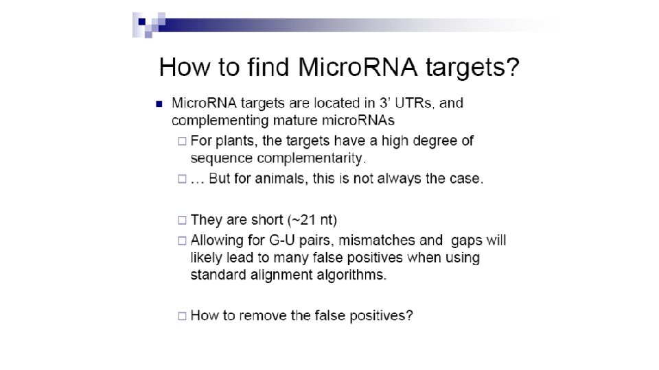
Finding mi. RNA Targets: Method 1 • Now we know of some mi. RNAs, but where do they attack? • Goal: Find the targets of a set of mi. RNAs that are shared between human and mouse. • Looking for the mi. RNA recognition element (MRE), not whole m. RNA. This is just the part that the mi. RNA would bind to. • Basic Assumption: Whole mi. RNA: MRE interactions (binding) are likely to have highly energetically favorable base pairing. • Basic Method: Look through the conserved 3' UTRs—this is where the MREs are most likely to be located—and try to make an alignment that minimizes the binding energy between the mi. RNA sequence and the UTRs (most favorable).

Finding mi. RNA Targets: Method 1 • Method: • First look at the binding energies of all 38 -mers of the m. RNA when binding to the mi. RNA. Subsequently apply several filters to pick alignments that “look” like mi. RNA binding. • Why 38 -mers? ~22 nt for the mi. RNA and the rest to allow for bulges, loops, etc. • Algorithm: Use a modified dynamic programming sequence alignment algorithm to calculate the binding energies for each 38 -mer. • Modifications: Scoring and speedup

Finding mi. RNA Targets: Method 1 • Scoring: • Mismatches and indels allowed. • Matrix based on RNA-RNA binding energies. • Use known binding energies of Watson-Crick pairing and wobble (G-U) pairing. • Binding energy (score) calculated for every two adjacent pairings (unlike the standard alignment algorithm which just takes into account the “score” for one pair at a time). • Adds dimensions to scoring matrix. • Adds complexity to recurrence relation.

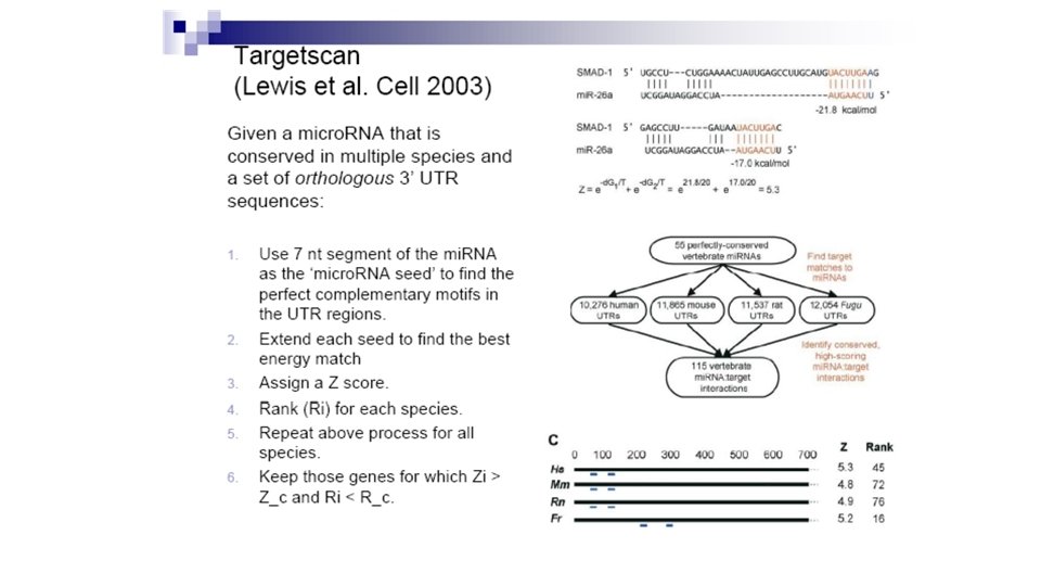
Finding mi. RNA targets: Method 2 • Goal: Find the set of mi. RNA targets for mi. RNAs shared across multiple species • Trying to identify which genes have 3' UTRs are attacked by mi. RNAs • Basic Assumptions: 1. There is perfect binding to the mi. RNA seed. 2. Any leftover sequence wants to achieve optimal RNA secondary structure. • Basic Method: For each species’ set of 3' UTRs, find sites where there is perfect binding of the mi. RNA seed and “optimal folding” nearby. Look for agreement among all the species.

Method 2: Example

Method 2: Steps 1. Find a perfect match to the mi. RNA seed. 2. Extend the matching region if possible. 3. Find the optimal folding for the remaining sequences. 4. Calculate the energy of this interaction.

Method 2: Details • Input: A set of mi. RNAs conserved among species and a set of 3' UTR sequences for those species. • Method: For each organism: 1. Find all occurrences in the UTR sequences that match the mi. RNA seed exactly. 2. Extend this region with perfect or wobble pairings. 3. With the remaining sequence of the mi. RNA, use the program RNAfold to find optimal folding with the next 35 bases of the UTR sequence. 4. Calculate a score for this interaction based on the free energy of the interaction given by RNAfold.

Method 2: Details • Method Cont. : 5. Sum up the scores of all interactions for each UTR. 6. Rank all the organism's gene's UTRs by this score (sum of all interactions in that UTR). 7. Repeat the above steps for each organism. 8. Create a cutoff score and a cutoff rank for the UTRs. 9. Select the set of genes where the orthologous genes across all the sampled species have UTR's that score and rank above this cutoff.

Method 2: Details • Verification: • Find the number of predicted binding sites per mi. RNA. • Compare it to number of binding sites for a randomly generated mi. RNA. • The result is much higher.

Analysis of the Two Methods • Method 1: • Good at identifying very strong, highly complementary mi. RNA targets. • Found gene targets with one mi. RNA binding site, failed to identify genes with multiple weaker binding sites. • Method 2: • Good at identifying gene targets that have many weaker interactions. • Fails to identify single-site genes.

Analysis of the Two Methods • Both Methods: • Speed is an issue. • Won't find targets that aren't in the 3' UTR of a gene. • We need more species sequenced! • • Conserved sequences are used to discover small RNAs. Conserved small RNAs are used to discover targets. Confidence in prediction of small RNAs and targets. Allows for broader scope with different combinations of species.

Results • Predicted a large portion of already known targets and provided direction for identifying undiscovered targets. • Found that it is more common that genes are regulated by multiple small RNAs. • Found that many small RNAs have multiple targets.

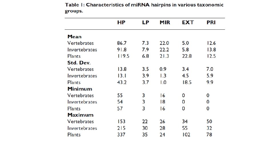
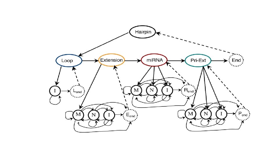
HHMMi. R: hierarchical HMMs for mi. R (Kadri et al 2009)

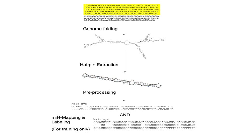
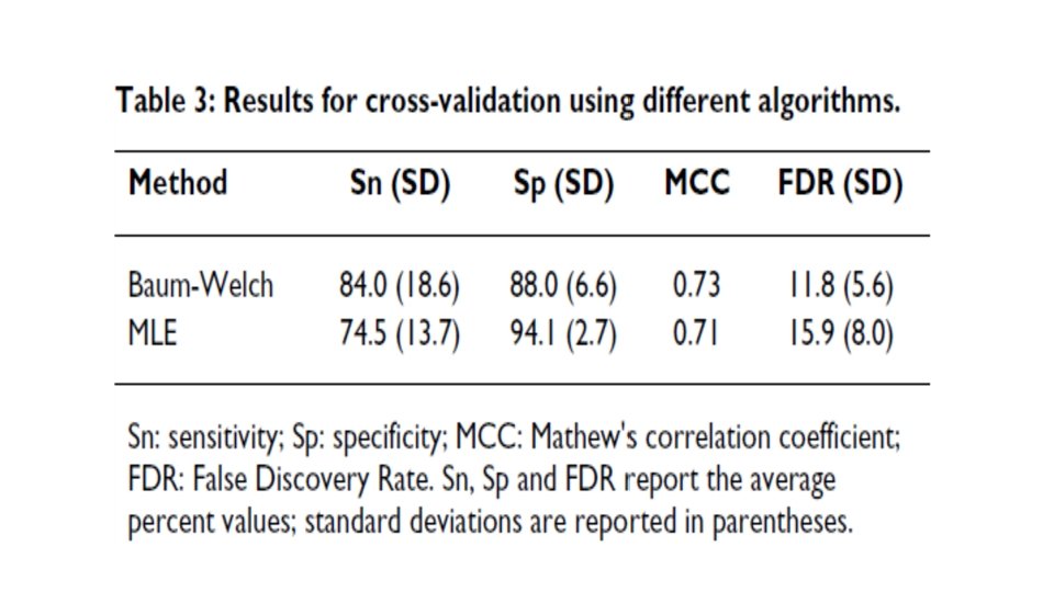
• Training: 527 human mi. RNA precursors (positive dataset) & ~500 random hairpins (negative dataset) • Hairpin processing… • Modified Baum/Welch and MLE

Various types of RNA • messenger RNA (m. RNA) • transfer RNA (t. RNA) • Ribosomal RNA (r. RNA) • small interfering RNA (si. RNA) • micro RNA (mi. RNA) • small nuclear RNA (sn. RNA) • small nucleolar RNA (sno. RNA)

Fabbri, The Cancer Journal, 14: 1, 2008

Outline • Introduction • history • mi. RNA biogenesis • Computational Methods • mature and precursor mi. RNA prediction • mi. RNA target gene prediction

Image: wiki

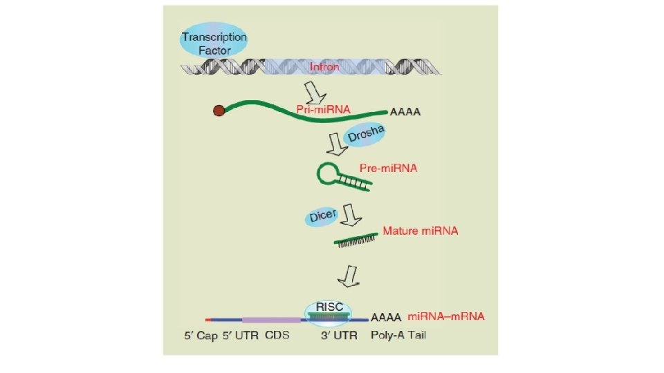
mi. RNA transcription and maturation

mi. RNA transcription and maturation 1. Nuclear gene to primary-mi. RNA 2. Cleavage to mi. RNA precursor by Drosha Rnase III 3. Transported to cytoplasm by Ran -GTP/Exportin 5 4. Loop cut by DICE 5. *duplex is short-lived and cut by helicase to single strand RNA forming RNA-induced silencing complex (RISC)/maturation Kadri et al 2009

Enabling machinery

3 examples of mi. RNAs • Size: 60 -80 bp premi. RNA • 2— 24 nt mature mi. RNA • Role: translation regulation, cancer diagnosis • Location: intergenic or intronic

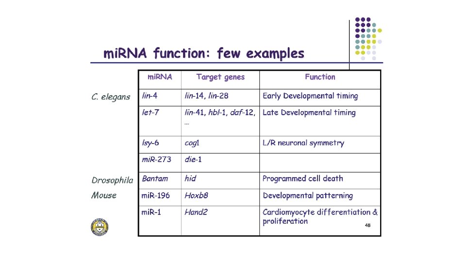
mi. RNA function

Challenging the dogma Mattick, Bio. Essays, 25: 930 -939, 2003.

• How to find micro. RNA genes? • Given a mi. RNA gene, how to find its targets? • Target-driven approach: • Xie et al (2005) analyzed conserved motifs overrepresented in 3’ UTR’s of genes • Motifs found to complement the sequences of known mi. RNAs • 120 new mi. RNAs predicted in humans

How to find mi. RNA gene? • Biological approach • Small RNA-cloning to identify new small RNAs • Most mi. RNA genes are tissue specific (picture) • mi. R-124 a is restricted to the brain and spinal cord in fish and mouse or to the ventral nerve cord in fly • mi. R-1 restricted to the muscles and the heart in the mouse

wiki

Principles of micro. RNA-m. RNA interactions Filipowicz et al Nature Reviews Genetics 2008

High-quality mi. RNAs story • mi. RBase: ~25 K entries; issues with quality

Need for computational methods • Experimental identification of mi. RNAs is slow because some mi. RNAs are difficult to isolate by cloning: • • Low expressions Instability Specific to tissue Trouble with cloning procedures • => computational methods can aid experiments

• 20 - to 24 -nt RNAs derived from endogenous transcripts that form local hairpin structures • Processing of mi. RNA leads to single (sometimes 2) mature mi. RNA molecules • Mature and pre-mi. RNA evolutionary conserved

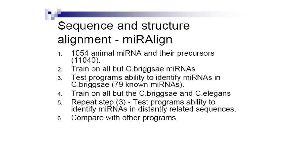
C. elegans mi. RNA genes • Scan for hairpin structures (RNAfold: free energy < -25 kcal/mole) within sequences that were conserved between C. elegans and C. briggsae (WU-BLAST cut-off E < 1. 8) • 36 K pairs of hairpins identified capturing 50/53 mi. RNAs previously reported to be conserved between the two species • 50 mi. RNAs used as training set for the program Mi. Rscan • Run mi. Rscan to evaluate 36 K hairpins

• Mi. Rscan evaluates features of a hairpin in a 21 -nt window • Total score = sum of individual feature scores • Scores are relative: frequency of the given value in the training set divided by the overall frequency Lim et al, Genes and Development, 2003 • mir-232 prediction circled in purple • 13. 9 total score

• • Blue: score distribution for 36 K sequences Red: training set of ~50 sequences Yellow and purple: verified by cloning and other evidence Green arrow: 13. 9

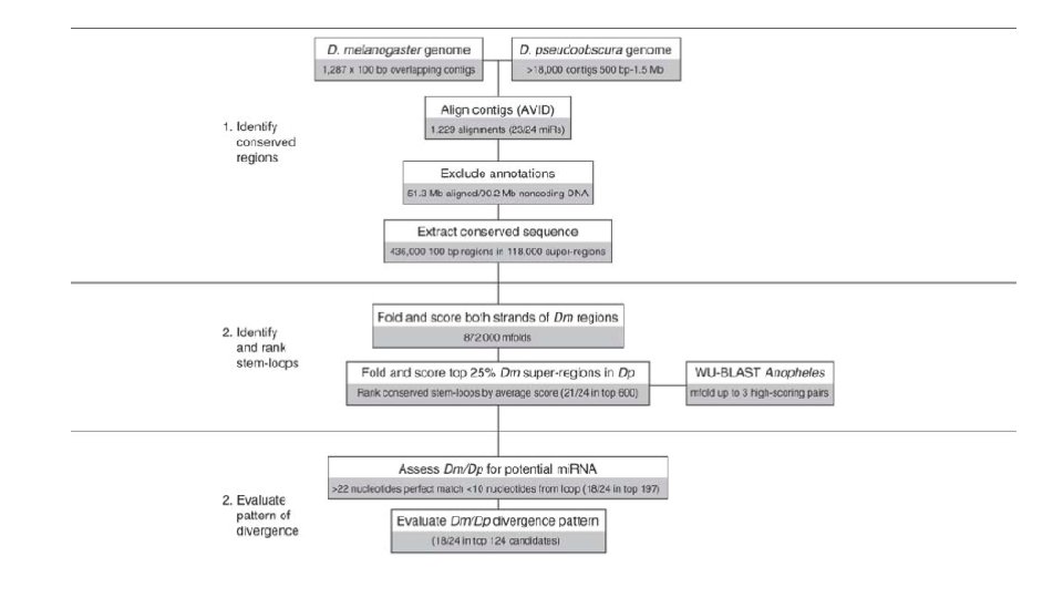
Drosophila mi. RNA genes • Two drosophila species: D. melanogaster and D. pseudoobscura • 3 -part computational pipeline: mi. Rseeker • Test on 24 known drosophila mi. RNAs

Drosophila m. RNA genes

Conserved stem-loop properties - 1

Conserved stem-loop properties -2

Results

Detection by homology • Entire set of human and mouse pre- and mature mi. RNA from the mi. RNA registry was submitted to the BLAT search engine to compare against both the human and mouse genomes • Sequences with high % identity were examined for hairpin structure using MFOLD and 16 -nt stretch base pairing

Found 60 new putative mi. RNAs (15: human and 45: mouse) • Mature mi. RNAs were either perfectly conserved or differed by 1 nt between human and mouse • Antisense mi. R: portion of the hairpin precursor that is base-paired with mi. R, as predicted by MFOLD

Drawbacks • Pipeline structure: use cut-offs and filtering/eliminating sequences as pipeline proceeds • Sequence alignment alone used to infer conservation (limited because areas of mi. RNA precursors are often not conserved) • Limited to closely related species (e. g. , C. elegans and C. briggsae)

Profile-based approach • 593 sequences form mi. RNA registry (513 animal and 50 plant) • CLUSTAL generated 18 most prominent mi. RNA clusters • Each cluster used to deduce consensus secondary structure using ALIFOLD program • Feed the training set to ERPIN: profile scan algorithm that reads sequence alignment and secondary structure • Scanned 14. 3 Gb database of 20 genomes

Results: 270/553 top scoring ERPIN candidates previously unidentified • Takes into account secondary structure conservation profiles • But only applicable to mi. RNA families with sufficient large known samples Legendre et al Bioinformatics, 2005

Use principles of micro. RNA-m. RNA interactions to predict targets Filipowicz et al Nature Reviews Genetics 2008

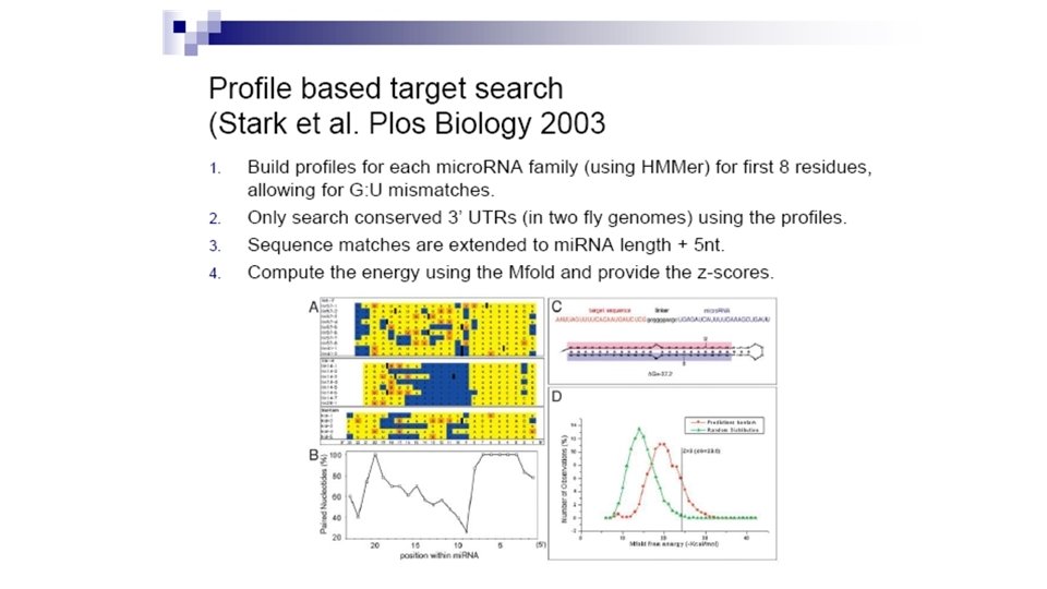
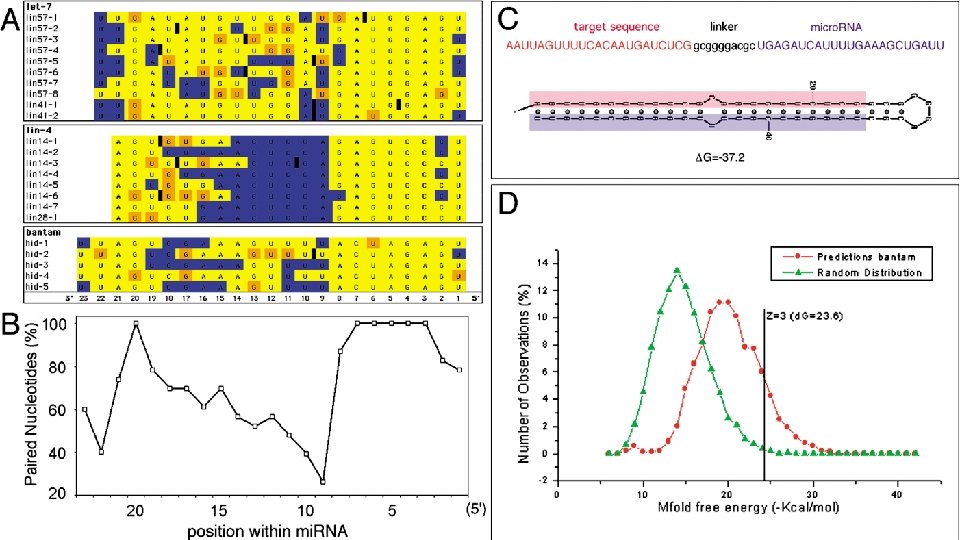
mi. RNA targets are often conserved across species (Stark et al PLo. S Biology, 2003) • For lins, compare C. elegans and c. briggsae • For hid, compare D. melanogaster and D. pseudoobscura

Other properties • Better complementarity to 5’ ends of mi. RNAs • Clusters of micro. RNA targets • Extensive co-occurrence of sites for different mi. RNAs in target 3’ UTR • Presence and absence of target sites correlates with gene function