METEOROLOGICAL PARAMETERS FROM SATELLITE IMAGERY CLOUD MOTION VECTORS

METEOROLOGICAL PARAMETERS FROM SATELLITE IMAGERY CLOUD MOTION VECTORS

WIND COVERAGE TRADITIONAL WEATHER BALLOONS

SATELLITE WINDS The idea of using successive satellite observations of clouds to determine wind direction and speed was pioneered by Professor Suomi of the University of Wisconsin-Madison. While the concept is simple, the procedure is rather complex.

Satellite Derived Winds Cover the globe and are available at multiple levels

BASIC PRINCIPLE 40 N/85 E 38. 5 N/83. 2 E

BASIC PRINCIPLE 40 N/85 E 38. 5 N/83. 2 E

BASIC PRINCIPLE ØA problem we have in tracking clouds is that we do not know the path they take Ø If we can determine the path they take we can determine the wind direction. Ø Watch the image of the car on the previous page and imagine that you did not have the roadway to help determine the car's path. Ø A good way to determine the path of the car is to track two images of the car that are close in time. Ø The same thinking applies to clouds. We view two images of a cloud that are close in time. Long time intervals are not good for tracking clouds that are changing rapidly. Short time intervals (1 to 15 minutes) are best when clouds are moving quickly.

Satellite Derived Winds • A sequence of Geo Stationery Sat images, separated by 15 or 30 minutes, are used to compute winds from satellite images. • This is particularly useful over the oceans where conventional weather observations are not possible. While it's true that buoys and ships send in weather observations they simply can't contribute anywhere near the coverage offered by satellites. • The accuracy of weather forecasts improved dramatically during the 1990's due to the addition of satellite derived winds in forecast models. This has been especially crucial to the timing and location of where a hurricane makes landfall.

Satellite Derived Winds The meteorological data on a global scale are so important for initialization purposes in Numerical Weather Prediction. Particularly over data-sparse areas like Indian Ocean, can be met only through derivation of products indirectly from satellite data. Satellites basically measure the radiance reaching them from the earth’s surface and cloud tops. By making such measurements in appropriate wavelengths applying physical and statistical techniques, it is possible to compute a wide range of products.

Some of the common parameters derived from the satellite images Atmospheric Motion Vectors (AMV) Outgoing Long wave Radiation (OLR) Quantitative Precipitation Estimates (QPE) Sea Surface Temperatures (SST)

Atmospheric Motion Winds (AMV) 1. Cloud Motion Vectors ( CMV) Using Visible Band Using Infrared band 2. Water Vapour Winds (WVW) Using Water Vapour Band

Basic Concept Derivation of a Wind Vector from the motion of the clouds. As we know that frequent images of the same area are only possible from the geostationary satellites. Therefore, by tracking the movement of the same cloud in successive images can give a good estimate of the winds

Basic Concept As shown in the figure , a cloud in image at time T is positioned at A( i, j ) and same cloud is positioned at B( i, j) in image at time T + T, then “A vector difference of the location of a cloud in two successive images divided by the time interval between images is an estimate of the horizontal wind at the level of the cloud” The difference between the two successive images could be 30 min, 7. 5 min or 3 min. The lesser value of difference can give more number of good quality winds.

Indian Geostationary Meteorological Satellites At present, there are three Indian Geostationary Meteorological Satellites. S. N. Name of Satellite 1. Kalpana – 1 2. INSAT – 2 E 3. INSAT – 3 A Year of Launch Position 2002 1999 2003 74°E 83°E 93. 5°E

Payloads on Kalpana – 1 S. N. Payload Channel Spectral Bandwidth 1. VHRR Resolution Visible 0. 55 - 0. 75 µ 2 Km. x 2 Km. 2. IR 10. 5 - 12. 5 µ 8 Km. x 8 Km. 3. Water Vapour 5. 7 - 7. 1 µ 8 Km. x 8 Km.

INSAT-2 E, INSAT-3 A Meteorological Payload : (i) VHRR (ii) CCD (i) VHRR Channels Spectral Range Resolution Visible 0. 55 - 0. 75 µ 2 Km. Infrared 10. 5 - 12. 5 µ 8 Km. Water Vapour 5. 7 - 7. 1 µ 8 Km. (ii) CCD Channels Visible NIR SWIR Spectral Range Resolution 0. 63 - 0. 69 µ 1 Km. 0. 77 - 0. 86 µ 1 Km. 1. 55 - 1. 69 µ 1 Km.

CLOUD MOTION VECTORS Cloud Motion Vectors are being derived both from Infrared and Visible data of Kalpana-1 & Insat-3 A Satellites from the triplets of following imagery : Time in UTC CMV’s From 1) 23: 30, 00: 00, 00: 30 IR Kalpana-1 2) 07: 00, 07: 30, 08: 00 IR, VIS Kalpana-1 3) 11: 30, 12: 00, 12: 30 IR Insat-3 A 4) 18: 00, 18: 30, 19: 00 IR Insat-3 A

STEPS IN THE COMUTATION OF CMV’s Ø In general, there are five steps in the derivation of Cloud Motion Vectors : o Registration of Triplet o Cloud Tracers selection o Tracking of Cloud Tracer in Target image o CMV Computation o Height Assignment Ø Quality Control of Cloud

1. Registration of Images Registration implies that when two images are displayed in time sequence, the land features should look stationary. In other words, two images are said to be registered if the landmarks in one image exactly overlay on the other image. The registration is achieved by shifting one image with respect to the other till the landmarks are lined up in both the images.

In Insat Meteorological Data Processing System (IMDPS), every reception is navigated automatically as a part of near real time processing. If required, the capabilities (NAVSHIFT) are applied which exercise the North. South or East-West translational shifts or rotation to achieve the accuracy of Navigation. It is presumed that frame to frame registration is achieved as result of accurate navigation and the computation of Vector Displacement uses latitude/longitude of the initial and final points of the Vector.

The steps of cloud tracer selection Ø Tracer Location List Generation Ø Tracer Threshold Calculation Ø Tracer Histogram Generation Ø Tracer Selection

f r e q u e n c y LOW CLEAR 0 0 MEDIUM HIGH pixel intensities 255 FOUR BIN HISTOGRAM FOR IR IMAGERY

Criteria For Tracer Selection At every selected location, a box of 16 x 16 pixels is 16 considered, Total Number of pixel in a box = 256 16 From the Four-Bin Histogram Total Number of low cloud pixels = Nc. L Total Number of medium cloud pixels = Ncm Total Number of high cloud pixels = Nch Total Number of cloudy pixels = Nc NC = NCL + NCM + NCH contd.

Criteria For Tracer Selection If the number of clear pixels contained in a box is equal to or greater than 85 % of total pixels, the box is treated as CLEAR (N - NC) > 85% of N If the number of cloudy pixels contained in a box is equal to or greater than 90 % of total pixels, the box is treated as CLOUDY NC > 90% of N Out of NCL , NCM and NCH , whichever is highest , the tracer is identified to be of that type.

TRACKING THE CLOUD TRACERS There are two basic methods of tracking of clouds v Manual Tracking v Automatic Tracking

Manual Tracking In this technique, an analyst locates the clouds to be tracked on each of two successive images. This is generally done by positioning a cursor at the cloud on a video display device. Advantages Even low clouds can be tracked through thin cirrus overcast. Theoretically, more number of vectors can be obtained. Disadvantages It is tedious and limits the number of tracers

Automatic Tracking In this method, individual clouds cannot be tracked. A pattern of clouds are tracked. Therefore, the average motion of an area of clouds is calculated. The automatic tracking is done primarily using the Cross Correlation method.

TRACKING THE CLOUD TRACERS CMV’s are being derived from two pairs of three half-hourly images at 0000 Z, 0730 Z , 1200 Z & 1800 Z CMV’s FROM 07: 30 Z CMV’s FROM TARGET IMAGE TRACER IMAGE 2330 0000 Z 0700 0730 TARGET IMAGE 0030 0800

Pattern Matching by Cross Correlation TRACER IMAGE TARGET IMAGE 16 16 (p, q) Best Fit Reference Window (T) Search Window (S) 1. Search window size for Low clouds is 36 2. Search window size for Medium clouds is 44 3. Search window size for High clouds is 52

Cross Correlation At each of the lag position (p, q), the cross correlation is calculated by the following formula N N (T(i, j) – T) (S(i+p, j+q) – S(p, q)) C(p, q)= i = 1 j=1 N N 2 (T(i, j) – T) i=1 j=1 N N (S(i+p, j+q)-S(p, q)) 2 i=1 j=1 Where T is the array of pixel intensities from the reference window and T is the mean, and S is the array of sub-set of search window at lag position (p, q) and S is the mean at that position The lag position (p, q) where the correlation coefficient is maximum is assumed to be the final position of the vector

MASKING OPTION Cloud tracking becomes difficult if multilayer clouds are present in the scene. overcome this difficulty, IMDPS To has a provision of ‘Masking Option’. All pixels in the reference and the Search window which were not identified as part of a specific cluster are masked out.

CLOUD MOTION VECTOR CALCULATION The CMV calculation is done in the following manner : (i) Target cloud classification / verification (ii) Vector Calculation

Target Cloud Classification/Verification This is basically a validation step so as to ensure that the same cloud pattern was tracked. For each of the tracked cloud targets, the four bin histogram is generated as was done for the cloud tracer and the same classification criteria is applied. The cloud target is rejected if it is not of the type of cloud tracer.

Vector Calculation The center of the reference / search window is the initial point of the vector and the location for which absolute maximum peak is obtained as the final position of the vector. From these positions, CMV is calculated. If correlation returns multiple locations with the same maximum value, the first one is accepted.

CMV Height Assignment Height assignment of the CMV’s is being done using Infrared Window (IRW) technique at present. Mean temperature of the 25% coldest IR pixels (John Le. Marshal et al. 1993, Merrill R 1989, Nieman S. J et al. 1997) is considered for assigning the height of the CMV. The software of the system is being upgraded and the H 2 O- IRW Intercept Method will also be tried shortly.

Problems in Height Assignment Problems are due to semitransparent clouds (such as cirrus) or sub pixel clouds (small clouds not filling the sensor field of view) Since the fraction of the sensor field of view occupied by the cloud is less than unity by an unknown amount, the brightness temperature Tb in the IR window is usually an overestimate of the cloud temperature. Thus, heights for semitransparent or subpixel clouds inferred directly from the observed Tb and an available temperature profile is consistently low

Quality Control Regarding quality control of the generated cloud motion vectors, the general approach is as follows: : v Reasonable Minimum and Maximum Limits of CMV v Testing the spatial and temporal consistencies of the vectors v Comparison of the vectors with forecast field vectors v Comparison with climatology in the event of nonavailability of forecast field

Editing of Cloud Motion Vectors OBJECTIVE QUALITY CONTROL • Absolute Threshold Test • Speed Test • Directional Stability Test • Gradient Test • Forecast Test • Climatology Test

Absolute Threshold Test A Target image at time T - 12 h VBA B C Target image at time T + 12 h Tracer image at time T VBC The two vectors (VBA and VBC ) generated from two pairs of images are individually checked for the limits of speeds possible for various cloud types i. e. |VBA| and |VBc| > Min. Speed, and |VBA| and |VBc| < Max. Speed

Speed Test In order to ensure that the two speeds do not have a large difference, this test is applied. | |VBA| - | VBc | | < 0. 5 Vaverage where Vaverage = | VBA | + | VBC | 2

Direction Stability Test This is basically to ensure temporal consistency. (i) If Vaverage < 20 Kts and the direction difference between VBA and VBc is more than 60 , the CMV is rejected (ii) If 60 > Vaverage > 20 and the direction difference between VBA and VBc is more than 40 , the CMV is rejected and (iii) If Vaverage > 60 Kts and the direction difference between VBA and VBc is more than 20 , the CMV is rejected.

RESULTANT VECTOR At this stage, the average VB of the two vectors viz. VBA and VBC is computed through U and V components which is then subjected to following tests. • Gradient Test • Forecast Field Test • Climatological Test

GRADIENT TEST Basically , this is to test horizontal consistency. (i) Speed difference between VB and the surrounding vectors must be less than the gradient speed threshold (20 kts). (ii) Direction difference between VB and surrounding vectors must be less than the gradient direction threshold (45 ). (iii) Distance from VB and the surrounding vectors must be less than the gradient distance threshold (300 Km. )

Forecast Field Test This is to test CMV’s against the forecast wind field produced by different centres of the world. At present, IMDPS CMV’s are being checked against the forecast field from Limited Area Model, IMD. v Speed difference between VB and the surrounding field must be less than 20 kts. v Direction difference between VB and the surrounding field must be less than 45 v Distance between VB and the surrounding field must be less than 300 Km.

Climatological Test If the forecast field is not available due to any reasons, the CMV’s are checked against climatology. The criteria of the test is same as that of forecast field.

Man-Machine Interactive Editing The CMV’s which have passed objective tests are available for interactive editing by the analyst at the work station. The CMV’s can be displayed on the monitor and the analyst can flag all those vectors which are inconsistent with the general field of motion. However, any deviant CMV can be retained if the cloud pattern suggest the likely existence of some new or rapidly changing circulation system. It is also possible to change the level of CMV.

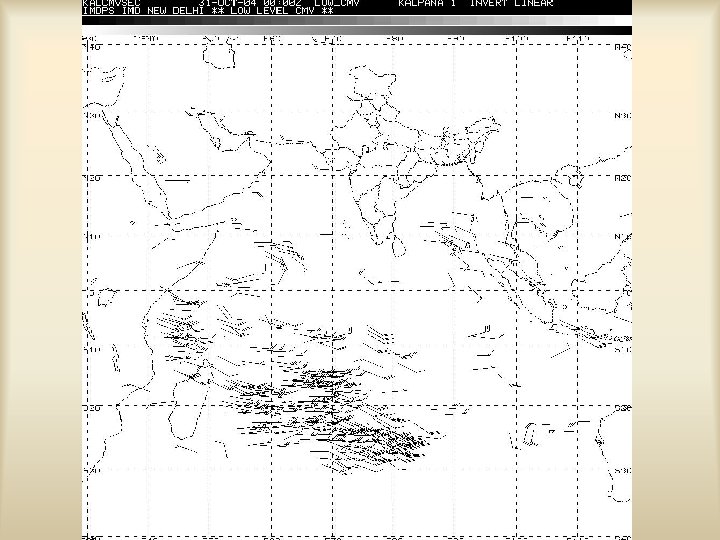
Low Level CMV’s Derived from Ir of Kalpana-1

Medium Level CMV’s Derived from Infrared of Kalpana-1 23 -May-04

High Level CMV’s Derived from Infrared of Kalpana-1 23 -May-04

Low. Level CMV’s From Visible Image of Kalpana – 1 : 29 -May-04

Medium Level CMV’s From Visible Image of Kalpana – 1 : 29 -May-04

High Level CMV’s From Visible Image of Kalpana – 1 : 29 -May-04

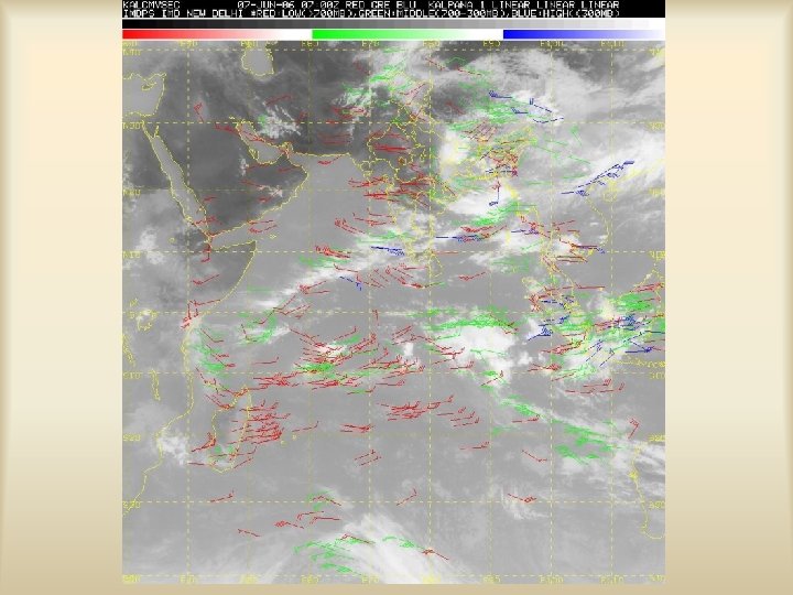
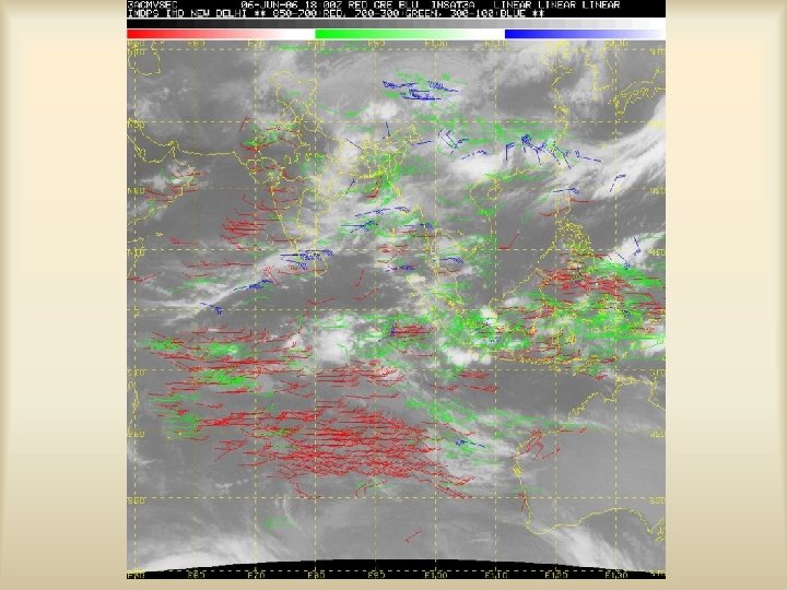
Low Level CMV’s From Visible Image of INSAT-3 A : 7 -JUNE-04

Medium Level CMV’s From Visible Image of INSAT-3 A : 7 -JUNE-04

High Level CMV’s From Visible Image of INSAT-3 A : 7 -JUNE-04

RAPID SCAN WINDS • INSAT Satellites have the capability to scan (Sector-Scan) a smaller area approx. 25 North-South in a span of 7 minutes repetitively three times. The Visible and Infrared images are shown in next slides.

Sector Scan VISIBLE Image from Kalpana-1

Sector Scan INFRARED Image from Kalpana-1

Sector Scan Low-Level CMV’s from IR data of Kalpana-1

Sector Scan Low-Level CMV’s from IR data of Kalpana-1

Sector Scan Med-Level CMV’s from IR data of Kalpana-1

Sector Scan High-Level CMV’s from IR data of Kalpana-1

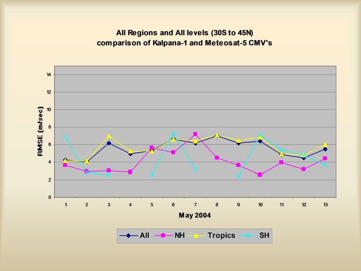
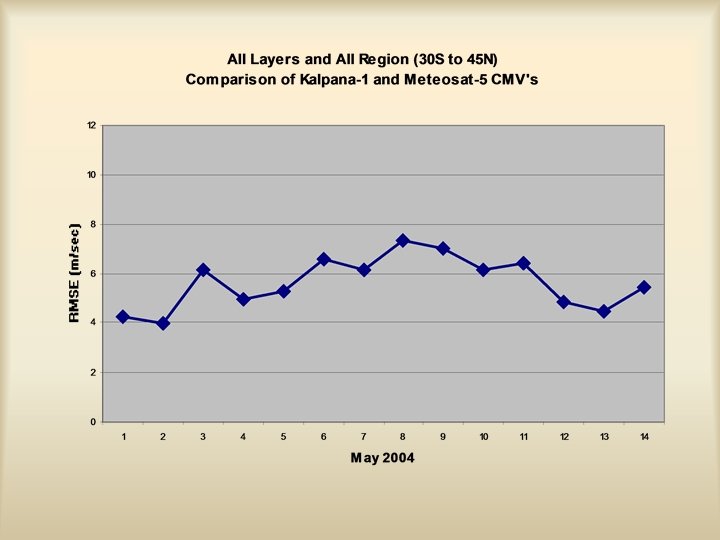
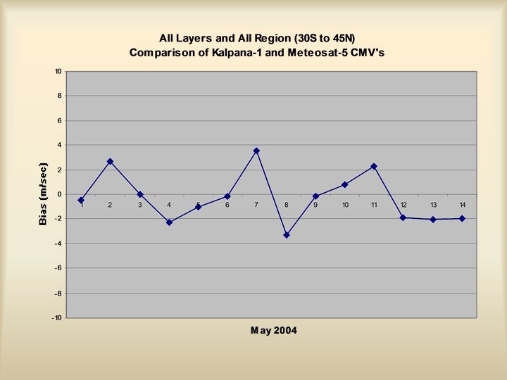
Validation of Cloud Motion Vectors The quantitative checks of the quality of CMV’s were made by comparing them with the first guess from Limited Area Model (LAM) Forecast field generated operationally by IMD. Monthly Statistics on rms errors and biases generated for the month of May 2004 is depicted in table-1. It is seen that for medium level CMVs, the bias of Kalpana-1 CMVs is 2. 0 m/sec or better. Rmse of Kalpana-1 CMVs is 6 m/sec for medium level CMVs which is fairly close to rmse of METEOSAT-5 CMVs. Same is the case with high level CMVs where rmse and biases have about 7 m/sec and 1. 5 m/sec respectively.

Table-1 ALL NH SH REGIONS EX-TROPICS ALL LEVELS MVD 5. 3 6. 0 5. 3 4. 9 RMSVD 6. 1 6. 8 6. 1 5. 8 STDVD 3. 1 3. 2 3. 1 3. 0 BIAS 2. 1 2. 0 2. 6 SPD 8. 9 7. 7 9. 0 9. 3 NUM 2835 310 2112 356 HIGH LEVEL MVD 6. 7 6. 6 6. 7 16. 3 RMSVD 7. 8 7. 9 7. 8 16. 3 STDVD 4. 0 4. 3 4. 0 0. 0 BIAS 3. 1 1. 6 3. 3 4. 2 SPD 12. 3 12. 5 12. 2 36. 5 NUM 244 20 221 1 ALL NH SH EX REGIONS EX-TROPICS MED. LEVEL MVD 5. 7 6. 2 5. 6 12. 6 RMSVD 6. 6 6. 9 6. 6 12. 7 STDVD 3. 4 3. 0 3. 5 1. 7 BIAS 2. 7 1. 9 2. 8 12. 0 SPD 8. 2 9. 0 8. 0 25. 2 NUM 537 88 440 3 LOW LEVEL MVD 5. 1 5. 8 5. 0 4. 8 RMSVD 5. 8 6. 6 5. 7 5. 6 STDVD 2. 8 3. 1 2. 7 2. 9 BIAS 1. 8 2. 1 1. 6 2. 5 SPD 8. 7 6. 7 8. 9 9. 1 NUM 2054 202 1451 352

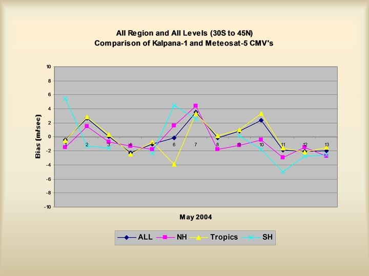
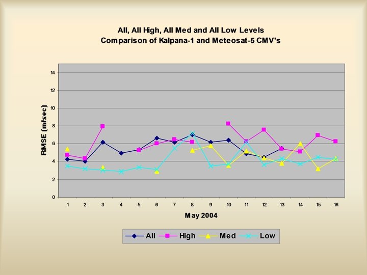
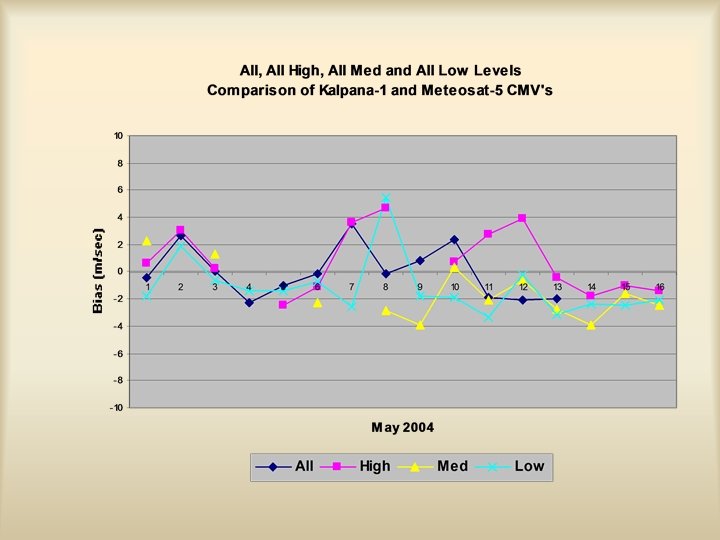
Comparison of Kalpana-1 CMV’s with METEOSAT-5 CMV’s

Table-2 ALL NH SH EX- REGIONS EX-TROPICS TROPICS ALL LEVELS RMSVD 5. 77 4. 05 6. 07 6. 13 BIAS 0. 48 1. 39 0. 27 0. 55 NCMV 93482 NC 2199 389 1723 87 HIGH LEVEL RMSVD 6. 65 -- 6. 59 6. 02 BIAS -0. 29 -- -0. 38 -0. 01 NCMV 69068 NC 1327 -- 1257 70 MED. LEVEL RMSVD 5. 09 4. 13 4. 75 6. 47 BIAS 1. 30 -2. 95 1. 97 1. 94 NCMV 10680 NC 104 14 68 22 LOW LEVEL RMSVD 3. 90 3. 41 4. 27 4. 71 BIAS 1. 67 1. 31 2. 03 -4. 19 NCMV 13734 NC 806 378 425 3

Comparison of INSAT and METEOSAT-5 CMV’s Cloud Motion Wind Collocation Statistics ( C M W ) Satellite in use : Kalpana-1 and Meteosat-5 Selected channel : IR Reporting Period : 1 May 2004 - 1100 HRS 0 MIN UTC 31 May 2004 - 2300 HRS 0 MIN UTC ALL N H TROPICS S H REGIONS EX-TROPICS 20 N-20 S EX-TROPICS ALL LEVELS RMSVD BIAS NCMV NC MED. LEVEL 5. 77 -0. 48 93482 2199 4. 05 -1. 39 6. 07 -0. 27 6. 13 -0. 55 389 1723 87 RMSVD BIAS NCMV NC 5. 09 -1. 30 10680 104 4. 13 2. 95 4. 75 -1. 97 6. 47 -1. 94 14 68 3. 90 -1. 67 13734 806 3. 41 -1. 31 4. 27 -2. 03 4. 71 4. 19 378 425 3 22 LOW LEVEL HIGH LEVEL RMSVD BIAS NCMV NC 6. 65 0. 29 69068 1327 ---- 6. 59 0. 38 1257 6. 02 0. 01 RMSVD BIAS NCMV NC 70 Differences (m/s) or (deg) RMSVD = Vector Difference RMS BIAS = Speed Bias NCMV = No. of disseminated Meteosat-5 Winds NC = No. of Collocations Cloud Motion Wind Collocation Statistics

THE MET. OFFICE CGMS SATELLITE WIND STATISTICS The following statistics are derived for the satellite/channel combination shown, for the period indicated. They are observation - background field differences, where the background field is the LAM model field used in quality control. KALPANA-1 IR RMSE AND BIAS FOR MAY 2004 ALL NH SH REGIONS EX-TROPICS ALL LEVELS MVD 5. 3 6. 0 5. 3 4. 9 RMSVD 6. 1 6. 8 6. 1 5. 8 STDVD 3. 1 3. 2 3. 1 3. 0 BIAS 2. 1 2. 0 2. 6 SPD 8. 9 7. 7 9. 0 9. 3 NUM 2835 310 2112 356 MED. LEVEL MVD 5. 7 6. 2 5. 6 12. 6 RMSVD 6. 6 6. 9 6. 6 12. 7 STDVD 3. 4 3. 0 3. 5 1. 7 BIAS 2. 7 1. 9 2. 8 12. 0 SPD 8. 2 9. 0 8. 0 25. 2 NUM 537 88 440 3 HIGH LEVEL LOW LEVEL MVD 5. 1 5. 8 5. 0 4. 8 RMSVD 5. 8 6. 6 5. 7 5. 6 STDVD 2. 8 3. 1 2. 7 2. 9 BIAS 1. 8 2. 1 1. 6 2. 5 SPD 8. 7 6. 7 8. 9 9. 1 NUM 2054 202 1451 352 MVD 6. 7 6. 6 6. 7 16. 3 RMSVD 7. 8 7. 9 7. 8 16. 3 STDVD 4. 0 4. 3 4. 0 0. 0 BIAS 3. 1 1. 6 3. 3 4. 2 SPD 12. 3 12. 5 12. 2 36. 5 NUM 244 20 221 1 Notes: Satellite wind minus LAM model background field MVD = Mean vector difference RMSVD = RMS vector difference STDVD = Standard deviation of the vector difference BIAS = Average speed difference SPD = Averaged satellite wind speed NUM = Number of satellite winds received Boundaries: NH=north of 20 N, TR=20 N-20 S, SH=south of 20 S High=10 -400 h. Pa, Med. =401 -700 h. Pa, Low=701 -1000 h. Pa Derivation of statistics are as outlined in Report from the Working Group on Verification Statistics, Proc. Conf. 3 rd Int. Winds Workshop, p. 17, Ascona, Switzerland, 10 -12 June 1996, EUMETSAT, Darmstadt. Produced by Dr. Devendra Singh, Director Satellte Division, IMD, New Delhi

ONSET OF MONSOON 6 -8 JUNE 2003

Case 1: 05 -09 June 2003 Southwest monsoon advanced into Kerala (extreme southern part of India) and adjoining parts of Tamil Nadu on 8 th June with a delay of about a week. It advanced into parts of coastal and south interior Karnataka and some more parts of Tamil Nadu on 10 th. In the present study the performance of the limited area model for the onset phase of the monsoon was investigated. In this case the impact of Cloud Motion Vector (CMV) data was exmined in the operational NWP model during the onset phase of Summer Monsoon over Kerala. The model forecasts are produced with the additional CMV data and compared with the operational real-time forecasts produced without this data. The 24 hours forecast rainfall based on the experiment for 8 th June shows the rainfall belt extending northwards over Kerala and Tamil Nadu. The 24 hours forecast rainfall based on the experiment for 8 th June shown slight northward propagation in the rainfall belt compared to the control run (Fig. 14) that agrees better with the observations. Verification analysis and forecast fields with this additional data has shown substantial improvements in the analysis and model predicted rainfall.

06 JUNE 2003 08 JUNE 2003 07 JUNE 2003 09 JUNE 2003 Fig. 1. KALPANA 1 VISIBLE (0600 Z) for 06, 07, 08 and 09 June 2003

Fig. 2. Analysis 700 h. Pa wind fields for 07, 08, 09 June 2003

Fig. 3. 24 Hrs Forecast 700 h. Pa wind fields control, experiment and analysis for 08 June 2003

Fig. 2. Model predicted 24 hours Rainfall (mm) for 08 June 2003 Left: Control, Right: Experiment

Case 2 18 May 2004 The onset of Monsoon of the year 2004 was also studied. The onset took place on 18 th May, 2004 about two weeks earlier than the normal onset date of 1 st June over Kerala. The limited area analysis and forecasts based on 18 th May 2004. The 700 h. Pa wind field shows the Southwesterly flow with wind strength of 20 -30 Kts. Over Southern parts of India and at 200 h. Pa the easterlies extending upto 15 N along the Southern peninsular India. The 24 hrs forecast for 19 th June shows the further strengthening of wind along the bay of Bengal and north east parts of India. The model predicted rainfall along the west coast and north-eastern parts of India was more realistic.

Fig. 1 Analysis - 700, 200 h. Pa Wind (kt) for 12 UTC of 18 -05 -2004

Fig. 2. 24 hrs Forecast - 700, 200 h. Pa Wind (kt) and Rainfall (mm) for 12 UTC of 19 -05 -2004

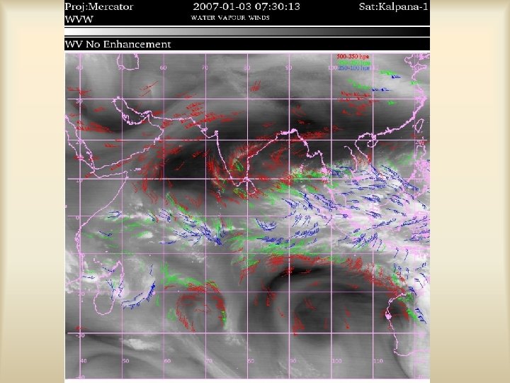
Water Vapour Winds (WVW)

THANK YOU !!!