K M A Korea Meteorological Administration NMSC National

K M A Korea Meteorological Administration NMSC National Meteorological satellite center GSICS Web. Meeting, 14 August 2013 DCC BRDF produced by SBDART model for COMS visible calibration Minjin CHOI National Meteorological Satellite Center / Korea Meteorological Administration Korea

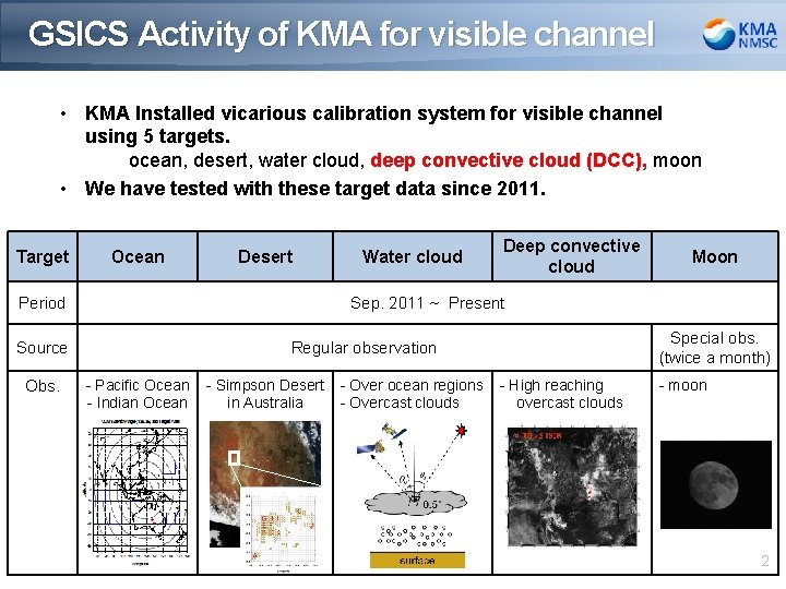
GSICS Activity of KMA for visible channel • KMA Installed vicarious calibration system for visible channel using 5 targets. ocean, desert, water cloud, deep convective cloud (DCC), moon • We have tested with these target data since 2011. Target Ocean Desert Period Deep convective cloud Moon Sep. 2011 ~ Present Source Obs. Water cloud Special obs. (twice a month) Regular observation - Pacific Ocean - Indian Ocean - Simpson Desert in Australia - Over ocean regions - Overcast clouds - High reaching overcast clouds - moon 2

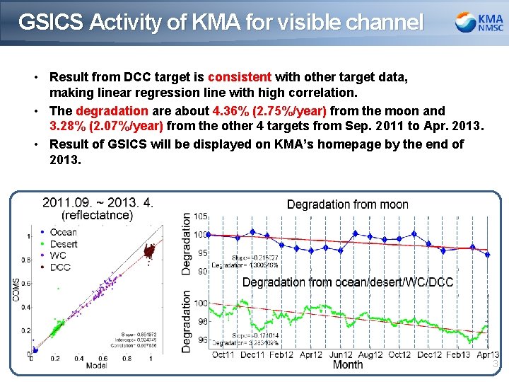
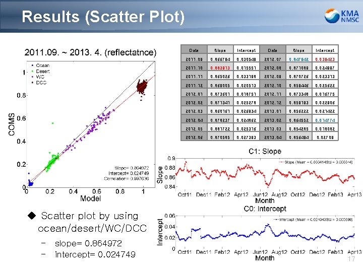
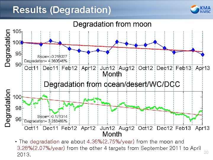
GSICS Activity of KMA for visible channel • Result from DCC target is consistent with other target data, making linear regression line with high correlation. • The degradation are about 4. 36% (2. 75%/year) from the moon and 3. 28% (2. 07%/year) from the other 4 targets from Sep. 2011 to Apr. 2013. • Result of GSICS will be displayed on KMA’s homepage by the end of 2013. 3

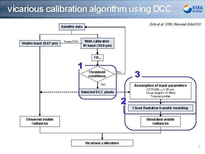
vicarious calibration algorithm using DCC Sohn et al. 2009, Ham and Sohn 2010 Satellite data Visible band (0. 67 μm) Same FOV Well-calibrated IR band (10. 8 μm) 1 TB 11 Threshold conditions No Yes Assumption of input parameters Selected DCC pixels 2 Observed visible radiances 3 COT=200, re = 20 μm, Cloud height = 1~15 km Tropical profiles Cloud Radiative transfer modeling Simulated visible radiances Vicarious calibration 4

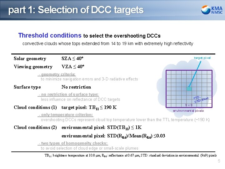
part 1: Selection of DCC targets Threshold conditions to select the overshooting DCCs convective clouds whose tops extended from 14 to 19 km with extremely high reflectivity Solar geometry SZA ≤ 40º Viewing geometry VZA ≤ 40º target pixel - geometry criteria: to minimize navigation errors and 3 -D radiative effects Surface type No restriction - no restriction of surface type: less influence on reflectance of DCC targets Cloud conditions (1) target pixel: TB 11 ≤ 190 K 9 x 9 , STD Mean / D ST environmental pixels - only temperature criterion: overshooting DCCs represent cloud top temperature lower than the TTL temperature (~190 K) Cloud conditions (2) environmental pixel: STD(TB 11) ≤ 1 K environmental pixel: STD(R 0. 6)/Mean(R 0. 6) ≤ 0. 03 - two types of homogeneity checks: to avoid selection of cloud edge or small-scale plumes TB 11: brightness temperature at 10. 8 μm, R 0. 6: reflectance at 0. 67 μm, STD: standard deviation in environmental (9 x 9) pixels 5

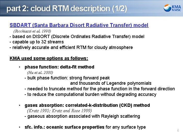
part 2: cloud RTM description (1/2) SBDART (Santa Barbara Disort Radiative Transfer) model (Ricchiazzi et al. 1998) - based on DISORT (Discrete Ordinates Radiative Transfer) model DISORT model - capable up to 32 streams - relatively accurate and efficient RTM for cloudy atmosphere KMA used some options as follows: • phase function: delta-fit method (Hu et al. 2000) - bulk phase function: strong forward peak and thousands of Legendre polynomials - needed to truncate method for the phase function in the forward direction - to reduce the computational burden without degrading accuracy • gases absorption: correlated-k-distribution (CKD) method (Kratz 1995; Kratz and Rose 1999) - gaseous absorption associated with Rayleigh scattering • sfc. info. : oceanic surface properties for any surface type 6

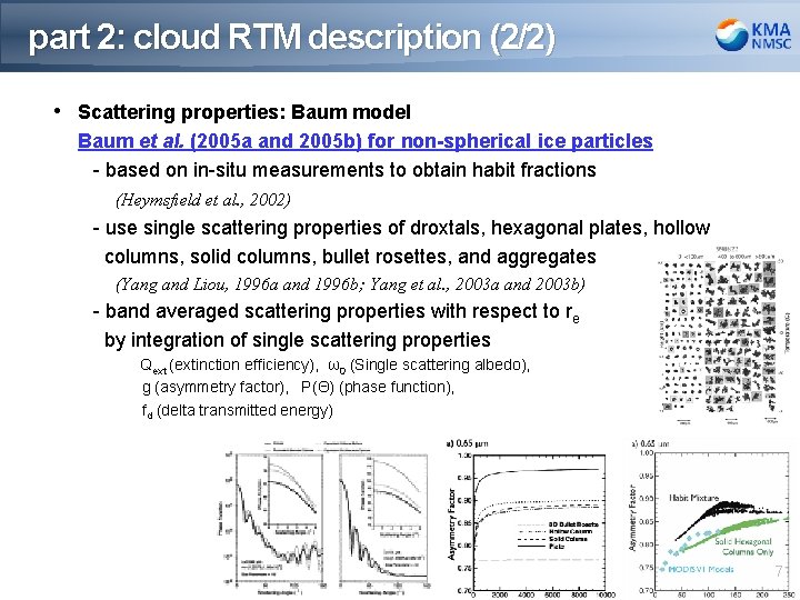
part 2: cloud RTM description (2/2) • Scattering properties: Baum model Baum et al. (2005 a and 2005 b) for non-spherical ice particles DISORT model - based on in-situ measurements to obtain habit fractions (Heymsfield et al. , 2002) - use single scattering properties of droxtals, hexagonal plates, hollow columns, solid columns, bullet rosettes, and aggregates (Yang and Liou, 1996 a and 1996 b; Yang et al. , 2003 a and 2003 b) - band averaged scattering properties with respect to re by integration of single scattering properties Qext (extinction efficiency), ω0 (Single scattering albedo), g (asymmetry factor), P(Θ) (phase function), fd (delta transmitted energy) 7

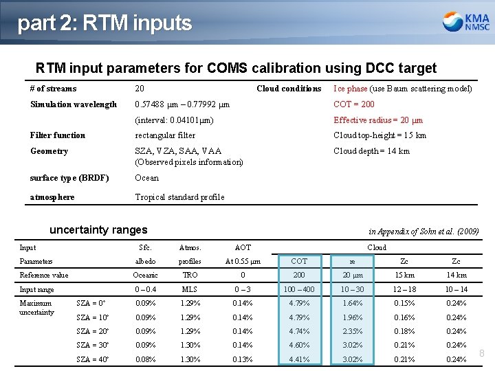
part 2: RTM inputs RTM input parameters for COMS calibration using DCC target # of streams 20 Cloud conditions Ice phase (use Baum scattering model) Simulation wavelength 0. 57488 μm – 0. 77992 μm COT = 200 (interval: 0. 04101μm) Effective radius = 20 μm Filter function rectangular filter Cloud top-height = 15 km Geometry SZA, VZA, SAA, VAA (Observed pixels information) Cloud depth = 14 km surface type (BRDF) Ocean atmosphere Tropical standard profile uncertainty ranges Input in Appendix of Sohn et al. (2009) Sfc. Atmos. AOT albedo profiles At 0. 55 μm COT re Zc Zc Reference value Oceanic TRO 0 20 μm 15 km 14 km Input range 0 – 0. 4 MLS 0– 3 100 – 400 10 – 30 12 – 18 10 – 14 SZA = 0º 0. 09% 1. 29% 0. 14% 4. 79% 1. 64% 0. 15% 0. 24% SZA = 10º 0. 09% 1. 29% 0. 14% 4. 79% 1. 96% 0. 16% 0. 24% SZA = 20º 0. 09% 1. 29% 0. 14% 4. 74% 2. 35% 0. 18% 0. 24% SZA = 30º 0. 09% 1. 30% 0. 14% 4. 60% 3. 02% 0. 21% 0. 24% SZA = 40º 0. 08% 1. 30% 0. 13% 4. 41% 3. 02% 0. 21% 0. 24% Parameters Maximum uncertainty Cloud 8

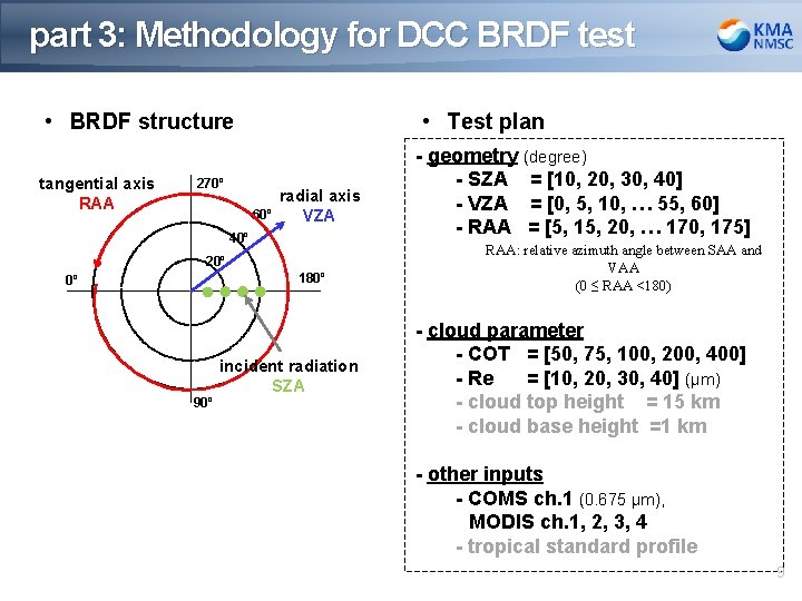
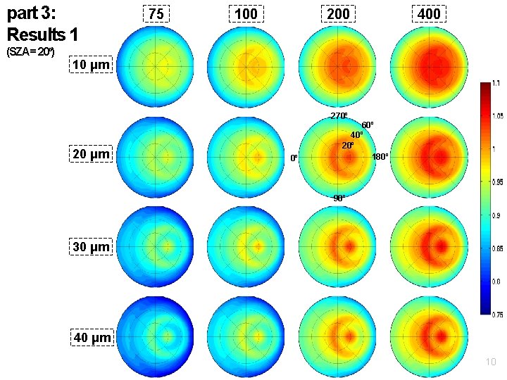
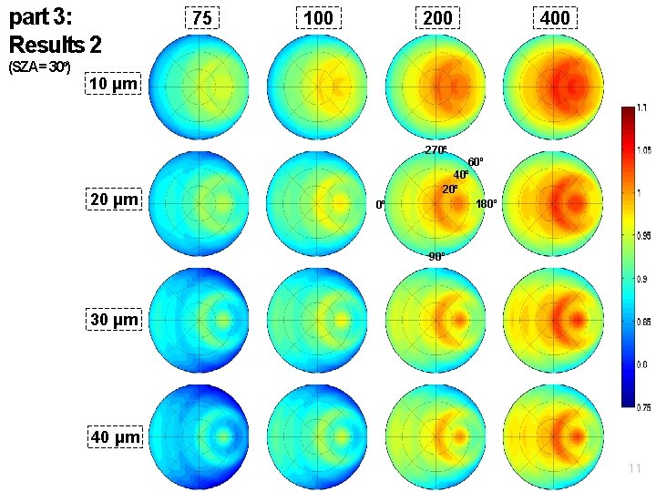
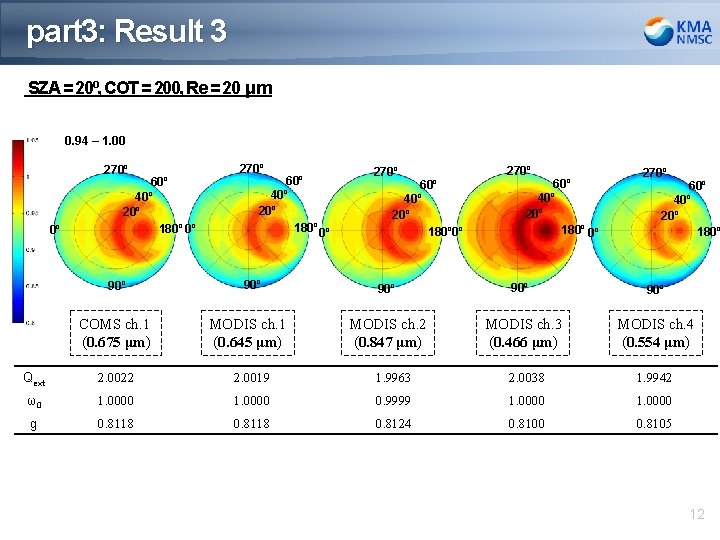
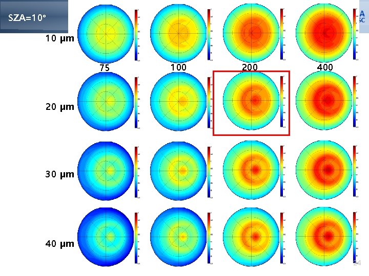
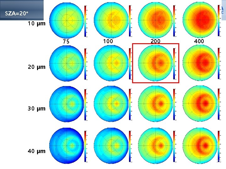
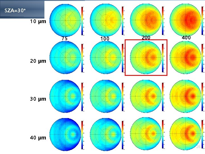
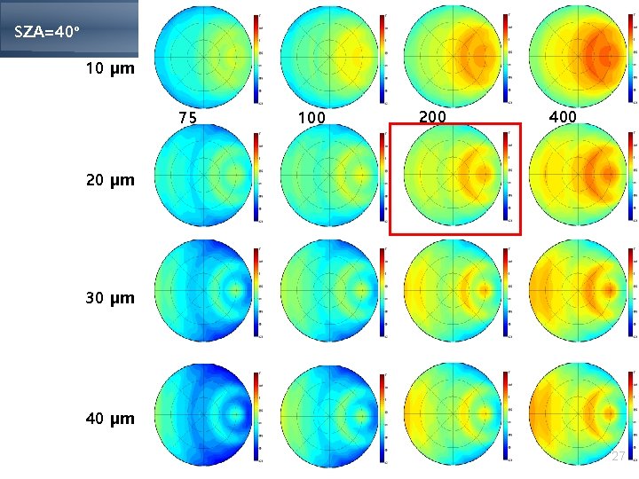
part 3: Methodology for DCC BRDF test • BRDF structure tangential axis RAA • Test plan 270º 60º radial axis VZA 40º 20º 180º 0º 90º incident radiation SZA - geometry (degree) - SZA = [10, 20, 30, 40] - VZA = [0, 5, 10, … 55, 60] - RAA = [5, 15, 20, … 170, 175] RAA: relative azimuth angle between SAA and VAA (0 ≤ RAA <180) - cloud parameter - COT = [50, 75, 100, 200, 400] - Re = [10, 20, 30, 40] (μm) - cloud top height = 15 km - cloud base height =1 km - other inputs - COMS ch. 1 (0. 675 μm), MODIS ch. 1, 2, 3, 4 - tropical standard profile 9

part 3: Results 1 (SZA = 20º) 75 100 200 400 10 μm 270º 20 μm 0º 60º 40º 20º 180º 90º 30 μm 40 μm 10

part 3: Results 2 (SZA = 30º) 75 100 200 400 10 μm 270º 20 μm 0º 60º 40º 20º 180º 90º 30 μm 40 μm 11

part 3: Result 3 SZA = 20º, COT = 200, Re = 20 μm 0. 94 – 1. 00 270º 0º 60º 40º 20º 180º 0º 90º COMS ch. 1 (0. 675 μm) 270º 60º 40º 20º 180º 0º 90º MODIS ch. 1 (0. 645 μm) 270º 90º 90º MODIS ch. 2 (0. 847 μm) MODIS ch. 3 (0. 466 μm) MODIS ch. 4 (0. 554 μm) 60º 40º 20º 180º 0º 270º 60º 40º 20º 180º Qext 2. 0022 2. 0019 1. 9963 2. 0038 1. 9942 ω0 1. 0000 0. 9999 1. 0000 g 0. 8118 0. 8124 0. 8100 0. 8105 12

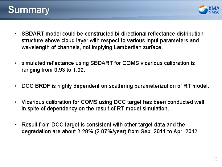
Summary • SBDART model could be constructed bi-directional reflectance distribution structure above cloud layer with respect to various input parameters and wavelength of channels, not implying Lambertian surface. • simulated reflectance using SBDART for COMS vicarious calibration is ranging from 0. 93 to 1. 02. • DCC BRDF is highly dependent on scattering parameterization of RT model. • Vicarious calibration for COMS using DCC target has been conducted well in spite of dependency on the result of RT model simulation. • Result from DCC target is consistent with other target data and the degradation are about 3. 28% (2. 07%/year) from Sep. 2011 to Apr. 2013. 13

Back-up slides 14

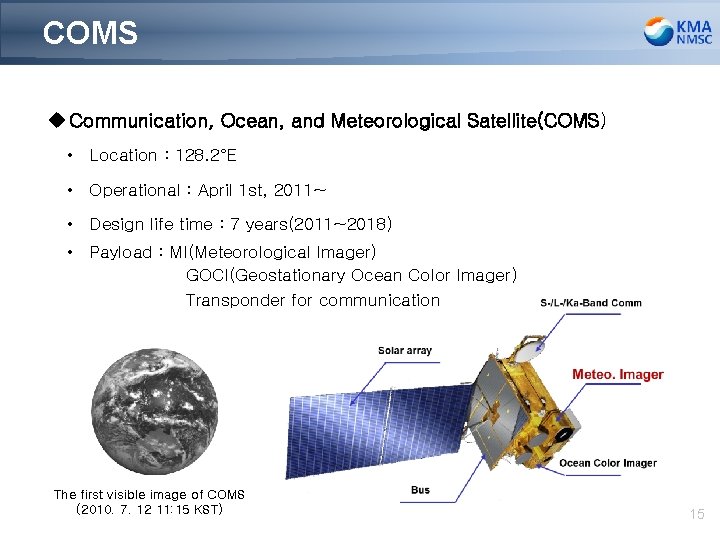
COMS u Communication, Ocean, and Meteorological Satellite(COMS) • Location : 128. 2°E • Operational : April 1 st, 2011~ • Design life time : 7 years(2011~2018) • Payload : MI(Meteorological Imager) GOCI(Geostationary Ocean Color Imager) Transponder for communication The first visible image of COMS (2010. 7. 12 11: 15 KST) 15

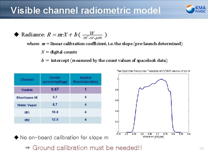
Visible channel radiometric model u Radiance: R = m∙X + b ( ) where m = linear calibration coefficient, i. e. the slope (pre-launch determined) X = digital counts b = intercept (measured by the count values of spacelook data) u No on-board calibration for slope m ⇒ Ground calibration must be needed!! 16

Results (Scatter Plot) Date Slope Intercept 2011. 09 0. 866794 0. 030549 2012. 07 0. 847942 0. 039423 2011. 10 0. 883913 0. 015551 2012. 08 0. 871089 0. 024997 2011. 11 0. 865026 0. 033198 2012. 09 0. 870726 0. 023313 2011. 12 0. 869005 0. 020513 2012. 10 0. 859446 0. 025622 2012. 01 0. 873601 0. 018751 2012. 11 0. 873348 0. 016775 2012. 02 0. 871341 0. 025278 2012. 12 0. 859193 0. 022906 2012. 03 0. 860161 0. 026934 2013. 01 0. 856222 0. 021422 2012. 04 0. 878237 0. 024862 2013. 02 0. 864552 0. 014774 2012. 05 0. 881722 0. 025316 2013. 03 0. 854285 0. 018082 2012. 06 0. 870585 0. 027393 2013. 04 0. 856494 0. 02709 u Scatter plot by using ocean/desert/WC/DCC - slope= 0. 864972 - intercept= 0. 024749 17

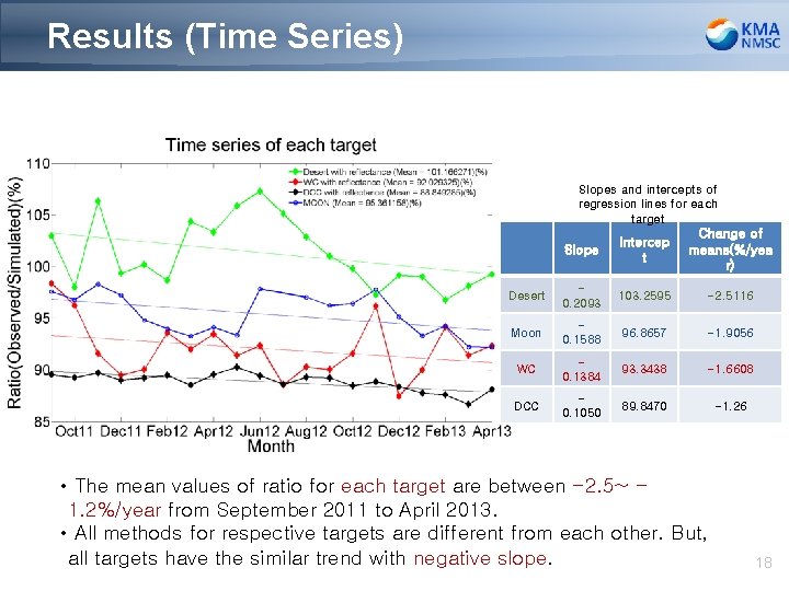
Results (Time Series) Slopes and intercepts of regression lines for each target Slope Intercep t Change of means(%/yea r) Desert 0. 2093 103. 2595 -2. 5116 Moon 0. 1588 96. 8657 -1. 9056 WC 0. 1384 93. 3438 -1. 6608 DCC 0. 1050 89. 8470 -1. 26 • The mean values of ratio for each target are between -2. 5~ 1. 2%/year from September 2011 to April 2013. • All methods for respective targets are different from each other. But, all targets have the similar trend with negative slope. 18

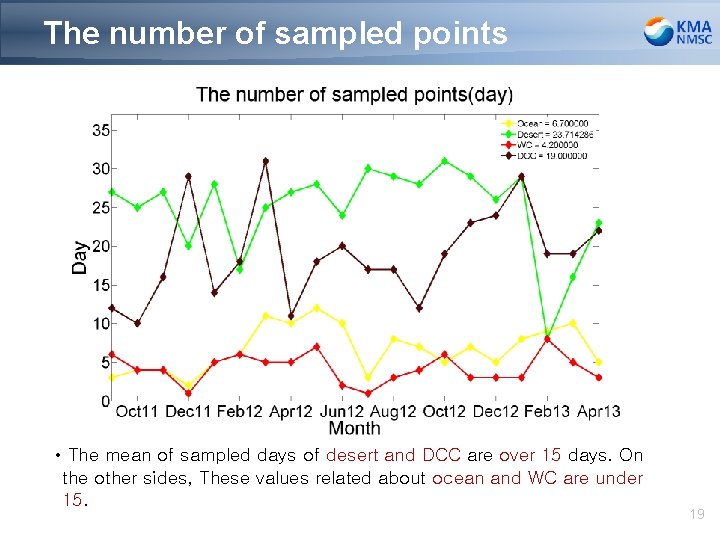
The number of sampled points • The mean of sampled days of desert and DCC are over 15 days. On the other sides, These values related about ocean and WC are under 15. 19

Results (Degradation) • The degradation are about 4. 36%(2. 75%/year) from the moon and 3. 28%(2. 07%/year) from the other 4 targets from September 2011 to April 2013. 20

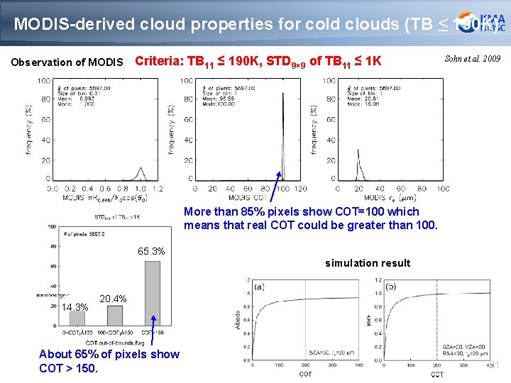
MODIS-derived cloud properties for cold clouds (TB ≤ 190 K) Observation of MODIS Criteria: TB 11 ≤ 190 K, STD 9× 9 of TB 11 ≤ 1 K Sohn et al. 2009 More than 85% pixels show COT=100 which means that real COT could be greater than 100. 65. 3% simulation result 14. 3% 20. 4% About 65% of pixels show COT > 150. 21

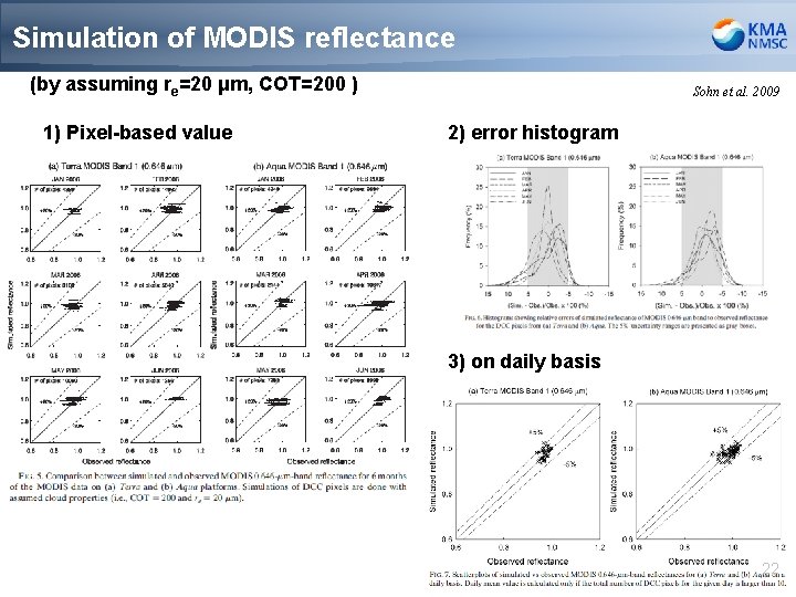
Simulation of MODIS reflectance (by assuming re=20 μm, COT=200 ) 1) Pixel-based value Sohn et al. 2009 2) error histogram 3) on daily basis 22

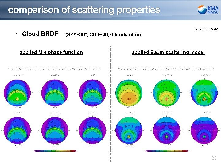
comparison of scattering properties • Cloud BRDF Ham et al. 2009 (SZA=30º, COT=40, 6 kinds of re) applied Mie phase function applied Baum scattering model 23

SZA=10º 10 μm 75 100 200 400 20 μm 30 μm 40 μm 24

SZA=20º 10 μm 75 100 200 400 20 μm 30 μm 40 μm 25

SZA=30º 10 μm 75 100 200 400 20 μm 30 μm 40 μm 26

SZA=40º 10 μm 75 100 200 400 20 μm 30 μm 40 μm 27