Satellites Since the early 1960 s virtually all

Satellites “Since the early 1960 s, virtually all areas of the atmospheric sciences have been revolutionized by the development and application of remote sensing techniques – that is , measurements of atmospheric properties and processes at a distance, using radiation. Storm sensors placed in space, on aircraft, and/or on the earth surface. ” Grant W. Petty

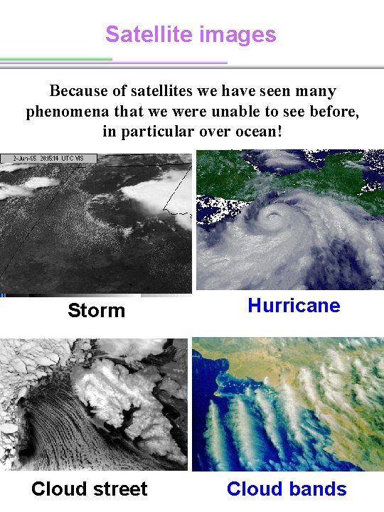
Satellite images Because of satellites we have seen many phenomena that we were unable to see before, in particular over ocean! Storm Cloud street Hurricane Cloud bands

Two major different types of satellites Geostationary vs. Polar-orbiting

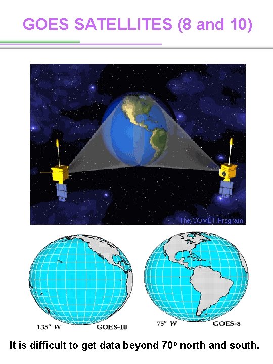
GOES SATELLITES (8 and 10) It is difficult to get data beyond 70 o north and south.

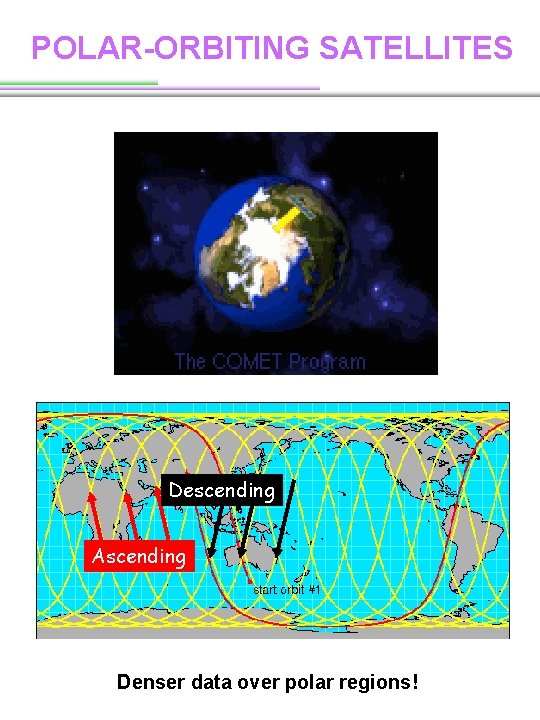
POLAR-ORBITING SATELLITES An inclination of 90 o Sun-Synchronous Orbit The orbit is a special case of polar orbiting (Satellites passing the same area approximately at the same local times every day) - Twice a day - To eliminate diurnal signal in data

POLAR-ORBITING SATELLITES Descending Ascending Denser data over polar regions!

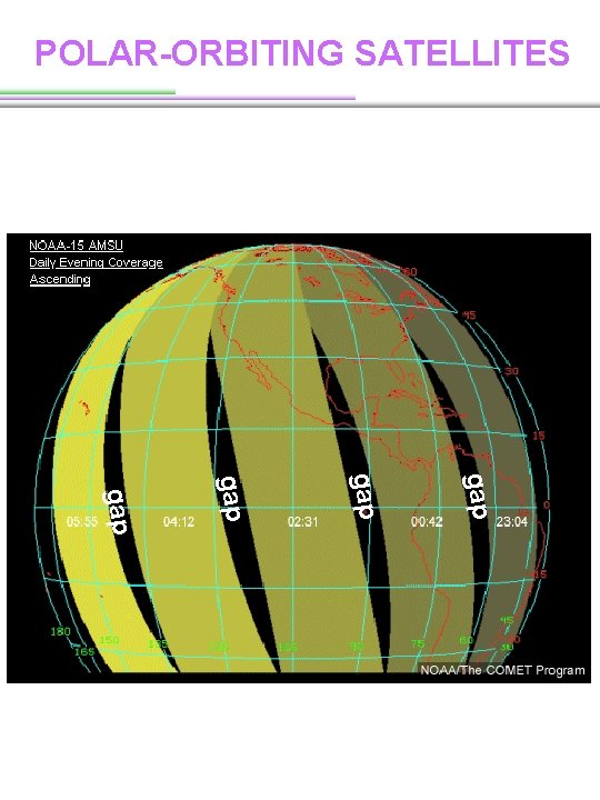
POLAR-ORBITING SATELLITES gap gap

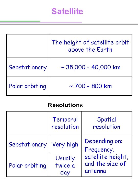
Satellite The height of satellite orbit above the Earth Geostationary ~ 35, 000 - 40, 000 km Polar orbiting ~ 700 - 800 km Resolutions Temporal resolution Geostationary Very high Polar orbiting Usually twice a day Spatial resolution Depending on: Frequency, satellite height, and the size of antenna

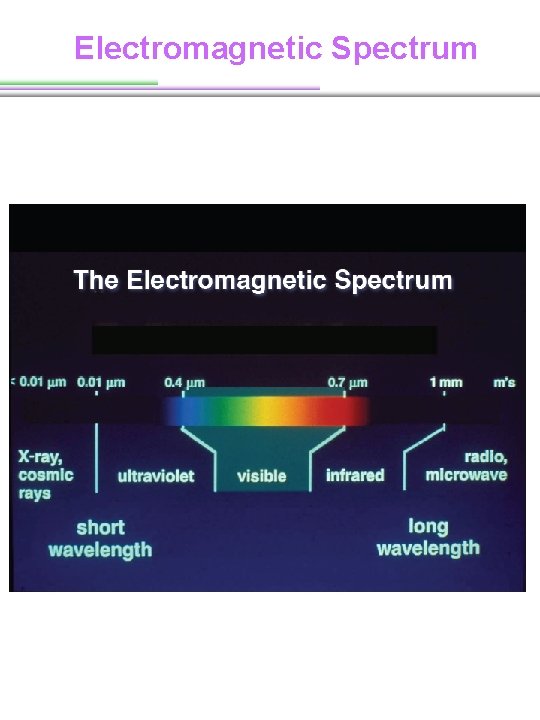
Electromagnetic Spectrum

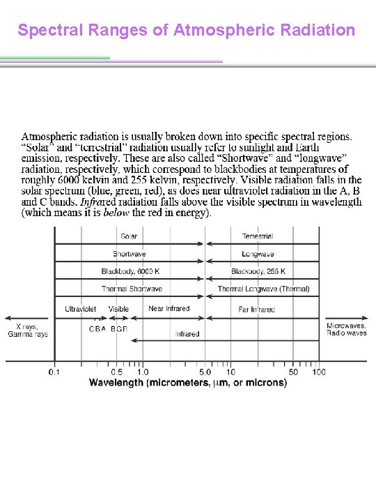
Spectral Ranges of Atmospheric Radiation

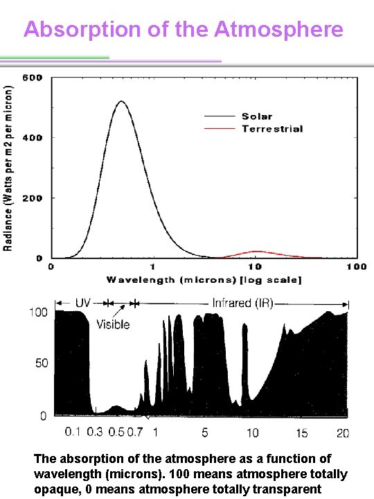
Absorption of the Atmosphere The absorption of the atmosphere as a function of wavelength (microns). 100 means atmosphere totally opaque, 0 means atmosphere totally transparent

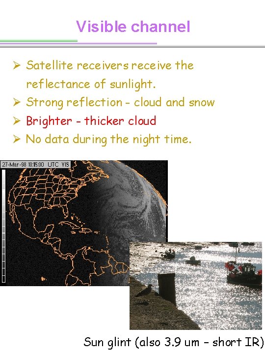
Visible channel Ø Satellite receivers receive the reflectance of sunlight. Ø Strong reflection - cloud and snow Ø Brighter - thicker cloud Ø No data during the night time. Sun glint (also 3. 9 um – short IR)

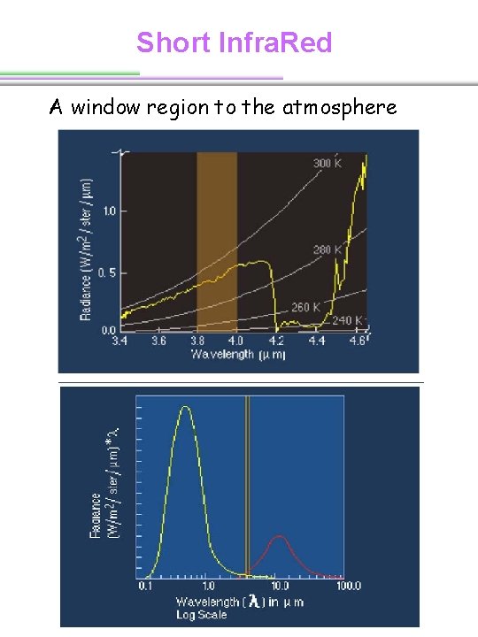
Short Infra. Red A window region to the atmosphere

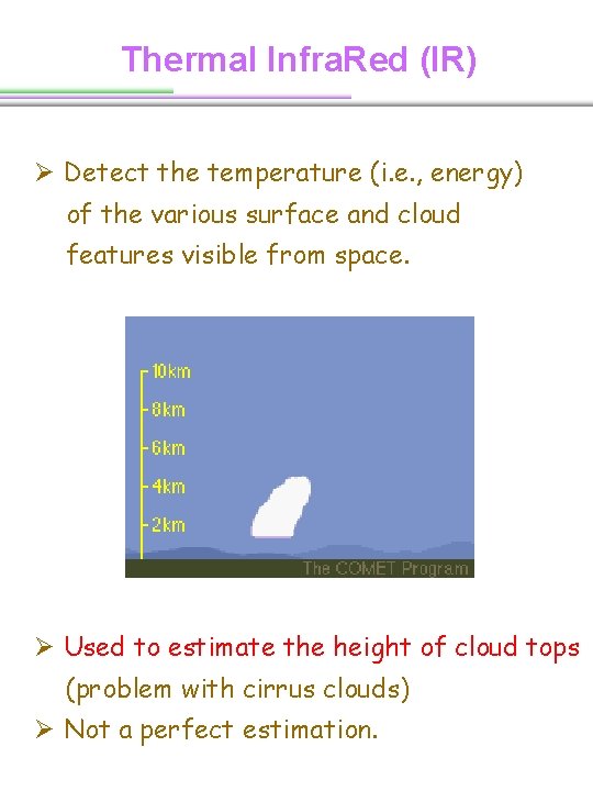
Thermal Infra. Red (IR) Ø Detect the temperature (i. e. , energy) of the various surface and cloud features visible from space. Ø Used to estimate the height of cloud tops (problem with cirrus clouds) Ø Not a perfect estimation.

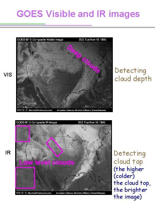
GOES Visible and IR images De ep VIS IR Low level clouds cl ou ds Detecting cloud depth Detecting cloud top (the higher (colder) the cloud top, the brighter the image)

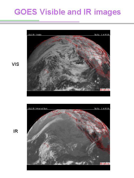
GOES Visible and IR images VIS IR

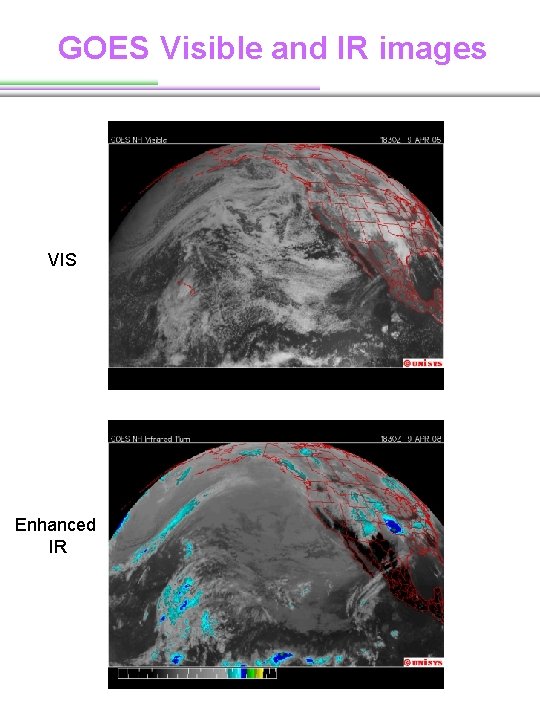
GOES Visible and IR images VIS Enhanced IR

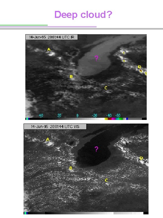
Deep cloud? ? ?

More satellites and Products

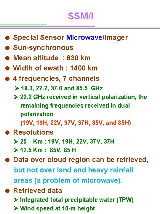
SSM/I = Special Sensor Microwave/Imager = Sun-synchronous = Mean altitude : 830 km = Width of swath : 1400 km = 4 frequencies, 7 channels 19. 3, 22. 2, 37. 0 and 85. 5 GHz 22. 2 GHz received in vertical polarization, the remaining frequencies received in dual polarization (19 V, 19 H, 22 V, 37 H, 85 V, and 85 H) = Resolutions 25 Km : 19 V, 19 H, 22 V, 37 H 12. 5 Km : 85 V, 85 H = Data over cloud region can be retrieved, but not over land heavy rainfall areas (a problem of microwave). = Retrieved data Integrated total precipitable water (TPW) Wind speed at 10 -m height

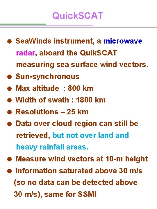
Quick. SCAT = Sea. Winds instrument, a microwave radar, aboard the Quik. SCAT measuring sea surface wind vectors. = Sun-synchronous = Max altitude : 800 km = Width of swath : 1800 km = Resolutions – 25 km = Data over cloud region can still be retrieved, but not over land heavy rainfall areas. = Measure wind vectors at 10 -m height = Information saturated above 30 m/s (so no data can be detected above 30 m/s), same for SSMI

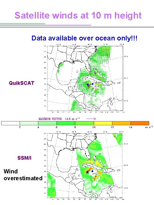
Satellite winds at 10 m height Data available over ocean only!!! Quik. SCAT SSM/I Wind overestimated

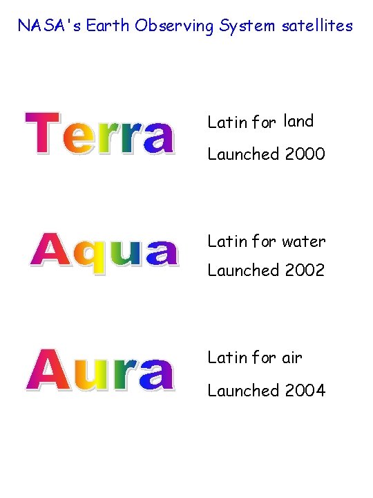
NASA's Earth Observing System satellites Latin for land Launched 2000 Latin for water Launched 2002 Latin for air Launched 2004

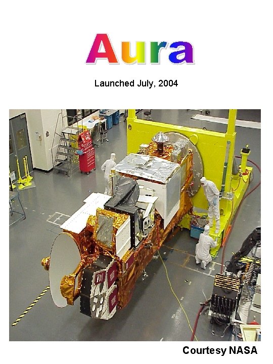
Launched July, 2004 Courtesy NASA

MODIS = Moderate Resolution Imaging Spectroradiometer = Aboard Terra (2000) and Aqua (2002) = 36 spectral bands: 0. 405 -14. 387 μm = Resolutions: 250 m, 500 m, 1000 m (radiances) = Sun-synchronous = Mean altitude : 705 km (equator) = Width of swath : 2300 km (Terra), 2330 (Aqua)

MODIS IR TPW Infra. Red (IR) – 5 km resolution • Derived from bands 24 to 36 (between 4. 47 to 14. 24 μm), excluding band 26 (data available day and night). • Used a statistical regression algorithm, with an option of a subsequent nonlinear physical retrieval (Seemann et al. 2003) => 101 -level atmospheric T, dew points, O 3 profiles, and skin T • 101 -level vertical T and dew point profiles = > TPW

MODIS n. IR TPW near Infra. Red (n. IR) – 1 km resolution • Used 2 water vapor absorption bands, 0. 905 and 0. 94 μm and 3 water vapor window bands, 0. 865, 0. 936, and 1. 24 μm. • Used a ratio of reflected solar radiances between an absorption channel to a window channel => water vapor transmittance • A pre-calculated water vapor transmittance look-up table = > TPW • The quality relies on water vapor attenuation of n. IR solar radiation reflected by surfaces and clouds. (daytime only)

MODIS n. IR TPW near Infra. Red (n. IR) – 1 km resolution • Over ocean, only sun glint regions can have data. • The accuracy of the data is strongly related to the estimation of surface reflection. (=>larger error over ocean)

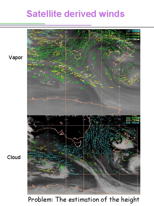
Satellite derived winds Vapor Cloud Problem: The estimation of the height

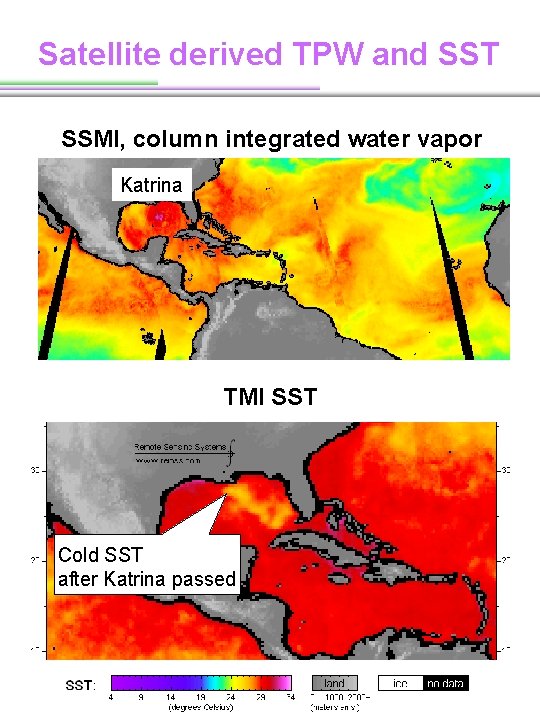
Satellite derived TPW and SST SSMI, column integrated water vapor Katrina TMI SST Cold SST after Katrina passed

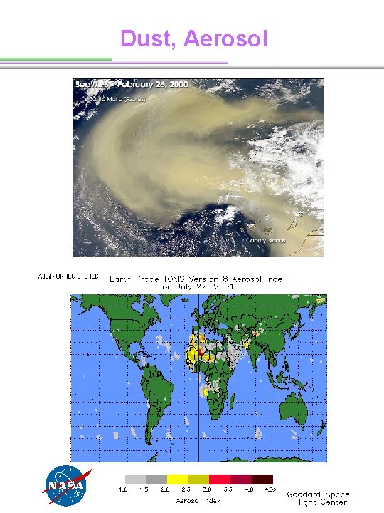
Dust, Aerosol

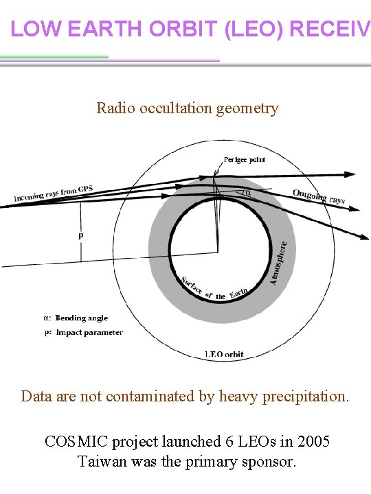
LOW EARTH ORBIT (LEO) RECEIV Radio occultation geometry Data are not contaminated by heavy precipitation. COSMIC project launched 6 LEOs in 2005 Taiwan was the primary sponsor.

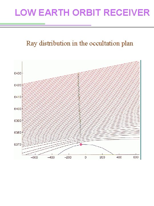
LOW EARTH ORBIT RECEIVER Ray distribution in the occultation plan

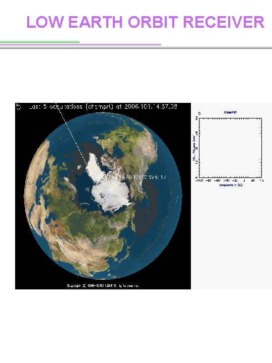
LOW EARTH ORBIT RECEIVER

Observations ØWhen using satellite data, need to know • What kinds of data? • The frequency of data • The resolution of data • The quality (or error) of data Ø What is the advantages and disadvantages of in situ and remote sensing data?