MATLAB PROGRAMMING MATLAB Tutorial Dr GUNASEKARAN THANGAVEL Lecturer

MATLAB PROGRAMMING MATLAB Tutorial Dr GUNASEKARAN THANGAVEL Lecturer & Program Co-ordinator Electronics & Telecommunication Engineering EEE Section Department of Engineering Higher College of Technology, Muscat. T. Gunasekaran MATLAB PROGRAMMING P. 1

MATLAB • Matlab = Matrix Laboratory • Originally a user interface for numerical linear algebra routines (Lapak/Linpak) • Commercialized 1984 by The Mathworks • Since then heavily extended (defacto-standard) Alternatives Complements • Matrix-X Octave Lyme Maple (symbolic) Mathematica (symbolic) T. Gunasekaran (free; GNU) (free; Palm) MATLAB PROGRAMMING P. 2

MATLAB • The MATLAB environment is command oriented somewhat like UNIX. A prompt appears on the screen and a MATLAB statement can be entered. When the <ENTER> key is pressed, the statement is executed, and another prompt appears. • If a statement is terminated with a semicolon ( ; ), no results will be displayed. Otherwise results will appear before the next prompt. • The following slide is the text from a MATLAB screen. T. Gunasekaran MATLAB PROGRAMMING P. 3

MATLAB To get started, type one of these commands: helpwin, helpdesk, or demo » a=5; » b=a/2 b = 2. 5000 » T. Gunasekaran MATLAB PROGRAMMING P. 4

MATLAB Variable Names • Variable names ARE case sensitive • Variable names can contain up to 63 characters (as of MATLAB 6. 5 and newer) • Variable names must start with a letter followed by letters, digits, and underscores. T. Gunasekaran MATLAB PROGRAMMING P. 5

MATLAB Special Variables ans pi inf Na. N i and j eps realmin realmax T. Gunasekaran Default variable name for results Value of Not a number e. g. 0/0 i = j = Smallest incremental number The smallest usable positive real number The largest usable positive real number MATLAB PROGRAMMING P. 6

MATLAB Math & Assignment Operators Power Multiplication Division or NOTE: ^ or. ^ a^b * or. * a*b / or. / a/b or. ba 56/8 = 856 - (unary) + (unary) Addition + Subtraction Assignment = T. Gunasekaran or or a. ^b a. *b a. /b b. a a + b a - b a = b (assign b to a) MATLAB PROGRAMMING P. 7

Other MATLAB symbols >>. . . , % ; : T. Gunasekaran prompt continue statement on next line separate statements and data start comment which ends at end of line (1) suppress output (2) used as a row separator in a matrix specify range MATLAB PROGRAMMING P. 8

MATLAB Help System • Search for appropriate function • >> lookfor keyword • Rapid help with syntax and function definition • >> help function • An advanced hyperlinked help system is launched by • >> helpdesk • Complete manuals as PDF files T. Gunasekaran MATLAB PROGRAMMING P. 9

MATLAB Matrices • MATLAB treats all variables as matrices. For our purposes a matrix can be thought of as an array, in fact, that is how it is stored. • Vectors are special forms of matrices and contain only one row OR one column. • Scalars are matrices with only one row AND one column T. Gunasekaran MATLAB PROGRAMMING P. 10

MATLAB Matrices • A matrix with only one row AND one column is a scalar. A scalar can be created in MATLAB as follows: » a_value=23 a_value = 23 T. Gunasekaran MATLAB PROGRAMMING P. 11

MATLAB Matrices • A matrix with only one row is called a row vector. A row vector can be created in MATLAB as follows (note the commas): » rowvec = [12 , 14 , 63] rowvec = 12 14 63 T. Gunasekaran MATLAB PROGRAMMING P. 12

MATLAB Matrices • A matrix with only one column is called a column vector. A column vector can be created in MATLAB as follows (note the semicolons): » colvec = [13 ; 45 ; -2] colvec = 13 45 -2 T. Gunasekaran MATLAB PROGRAMMING P. 13

MATLAB Matrices • A matrix can be created in MATLAB as follows (note the commas AND semicolons): » matrix = [1 , 2 , 3 ; 4 , 5 , 6 ; 7 , 8 , 9] matrix = 1 2 3 4 5 6 7 8 9 T. Gunasekaran MATLAB PROGRAMMING P. 14

Extracting a Sub-Matrix • A portion of a matrix can be extracted and stored in a smaller matrix by specifying the names of both matrices and the rows and columns to extract. The syntax is: sub_matrix = matrix ( r 1 : r 2 , c 1 : c 2 ) ; where r 1 and r 2 specify the beginning and ending rows and c 1 and c 2 specify the beginning and ending columns to be extracted to make the new matrix. T. Gunasekaran MATLAB PROGRAMMING P. 15

MATLAB Matrices • A column vector can be extracted from a matrix. As an example we create a matrix below: • Here we extract column 2 of the matrix and make a column vector: » matrix=[1, 2, 3; 4, 5, 6; 7, 8, 9] » col_two=matrix( : , 2) matrix = col_two = 1 2 3 4 5 6 7 8 9 2 5 8 T. Gunasekaran MATLAB PROGRAMMING P. 16

MATLAB Matrices • A row vector can be extracted from a matrix. As an example we create a matrix below: » matrix=[1, 2, 3; 4, 5, 6; 7, 8, 9] matrix = 1 2 3 4 5 6 7 8 9 T. Gunasekaran • Here we extract row 2 of the matrix and make a row vector. Note that the 2: 2 specifies the second row and the 1: 3 specifies which columns of the row. » rowvec=matrix(2 : 2 , 1 : 3) rowvec = 4 5 6 MATLAB PROGRAMMING P. 17

Reading Data from files • MATLAB supports reading an entire file and creating a matrix of the data with one statement. >> load mydata. dat; % loads file into matrix. % The matrix may be a scalar, a vector, or a % matrix with multiple rows and columns. The % matrix will be named mydata. >> size (mydata) % size will return the number % of rows and number of % columns in the matrix >> length (myvector) % length will return the total % no. of elements in myvector T. Gunasekaran MATLAB PROGRAMMING P. 18

Plotting with MATLAB • MATLAB will plot one vector vs. another. The first one will be treated as the abscissa (or x) vector and the second as the ordinate (or y) vector. The vectors have to be the same length. • MATLAB will also plot a vector vs. its own index. The index will be treated as the abscissa vector. Given a vector “time” and a vector “dist” we could say: >> plot (time, dist) % plotting versus time >> plot (dist) % plotting versus index T. Gunasekaran MATLAB PROGRAMMING P. 19

Plotting with MATLAB • There are commands in MATLAB to "annotate" a plot to put on axis labels, titles, and legends. For example: >> % To put a label on the axes we would use: >> xlabel ('X-axis label') >> ylabel ('Y-axis label') >> % To put a title on the plot, we would use: >> title ('Title of my plot') T. Gunasekaran MATLAB PROGRAMMING P. 20

Plotting with MATLAB • Vectors may be extracted from matrices. Normally, we wish to plot one column vs. another. If we have a matrix “mydata” with two columns, we can obtain the columns as a vectors with the assignments as follows: >> first_vector = mydata ( : , 1) ; >> second_vector = mydata ( : , 2) ; >>% and we can plot the data >> plot ( first_vector , second_vector ) T. Gunasekaran MATLAB PROGRAMMING % First column % Second one P. 21

Some Useful MATLAB commands • • whos help lookfor • • what clear x y clc T. Gunasekaran List known variables plus their size Ex: >> help sqrt Help on using sqrt Ex: >> lookfor sqrt Search for keyword sqrt in m-files Ex: >> what a: List MATLAB files in a: Clear all variables from work space Clear variables x and y from work space Clear the command window MATLAB PROGRAMMING P. 22

Some Useful MATLAB commands • what List all m-files in current directory • dir List all files in current directory • ls Same as dir • type test Display test. m in command window • delete test Delete test. m • cd a: Change directory to a: • chdir a: Same as cd • pwd Show current directory • which test Display current directory path to test. m T. Gunasekaran MATLAB PROGRAMMING P. 23

MATLAB Relational Operators • MATLAB supports six relational operators. Less Than or Equal Greater Than or Equal To Not Equal To T. Gunasekaran < <= > >= == ~= MATLAB PROGRAMMING P. 24

MATLAB Logical Operators • MATLAB supports three logical operators. not and or T. Gunasekaran ~ & | % highest precedence % equal precedence with or % equal precedence with and MATLAB PROGRAMMING P. 25

MATLAB Logical Functions • MATLAB also supports some logical functions. xor (exclusive or) Ex: xor (a, b) Where a and b are logical expressions. The xor operator evaluates to true if and only if one expression is true and the other is false. True is returned as 1, false as 0. any (x) returns 1 if any element of x is nonzero all (x) returns 1 if all elements of x are nonzero isnan (x) returns 1 at each Na. N in x isinf (x) returns 1 at each infinity in x finite (x) returns 1 at each finite value in x T. Gunasekaran MATLAB PROGRAMMING P. 26

MATLAB Display formats • MATLAB supports 8 formats for outputting numerical results. format long format short e format long e format hex format bank format + format rat format short T. Gunasekaran 16 digits 5 digits plus exponent 16 digits plus exponent hexadecimal two decimal digits positive, negative or zero rational number (215/6) default display MATLAB PROGRAMMING P. 27

Matlab Selection Structures • An if - else structure in MATLAB. Note that elseif is one word. if expression 1 % is true % execute these commands elseif expression 2 % is true % execute these commands else % the default % execute these commands end T. Gunasekaran MATLAB PROGRAMMING P. 28

MATLAB Repetition Structures • A for loop in MATLAB for x = array for x = 1: 0. 5 : 10 % execute these commands end • A while loop in MATLAB while expression while x <= 10 % execute these commands end T. Gunasekaran MATLAB PROGRAMMING P. 29

Scalar - Matrix Addition » a=3; » b=[1, 2, 3; 4, 5, 6] b = 1 2 3 4 5 6 » c= b+a % Add a to each element of b c = 4 5 6 7 8 9 T. Gunasekaran MATLAB PROGRAMMING P. 30

Scalar - Matrix Subtraction » a=3; » b=[1, 2, 3; 4, 5, 6] b = 1 2 3 4 5 6 » c = b - a %Subtract a from each element of b c = -2 -1 0 1 2 3 T. Gunasekaran MATLAB PROGRAMMING P. 31

Scalar - Matrix Multiplication » a=3; » b=[1, 2, 3; 4, 5, 6] b = 1 2 3 4 5 6 » c = a * b % Multiply each element of b by a c = 3 6 9 12 15 18 T. Gunasekaran MATLAB PROGRAMMING P. 32

Scalar - Matrix Division » a=3; » b=[1, 2, 3; 4, 5, 6] b = 1 2 3 4 5 6 » c = b / a % Divide each element of b by a c = 0. 3333 0. 6667 1. 0000 1. 3333 1. 6667 2. 0000 T. Gunasekaran MATLAB PROGRAMMING P. 33

MATLAB Toolbox • MATLAB has a number of add-on software modules, called toolbox , that perform more specialized computations. Signal & Image Processing Signal Processing- Image Processing Communications - System Identification - Wavelet Filter Design Control Design Control System - Fuzzy Logic - Robust Control - µ-Analysis and Synthesis - LMI Control Model Predictive Control More than 60 toolboxes! T. Gunasekaran MATLAB PROGRAMMING P. 34

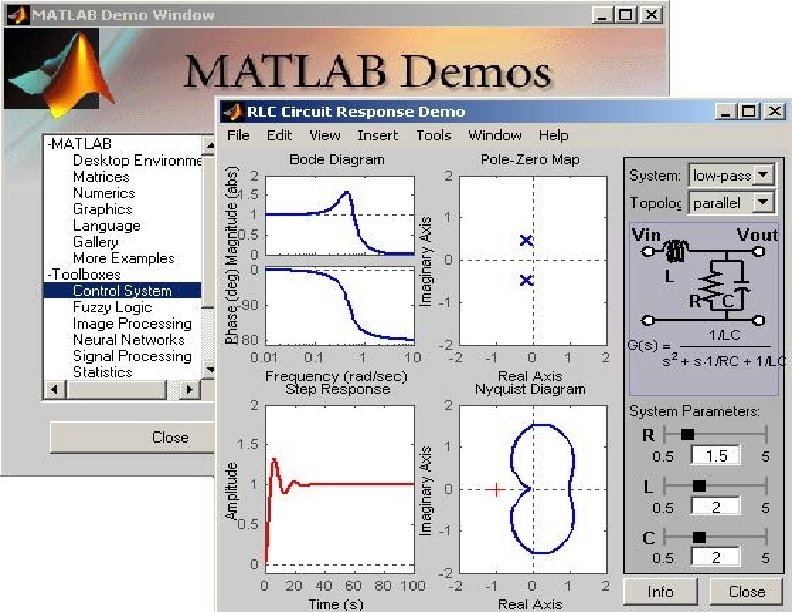
MATLAB Toolbox MATLAB has many toolboxes: • Control toolbox is one of the important toolbox in MATLAB. • RLC Circuit Response, • Gain and Phase Margins, • Notch Filter Discrete, • PID and. . . T. Gunasekaran MATLAB PROGRAMMING P. 35

MATLAB Demo • Demonstrations are invaluable since they give an indication of the MATLAB capabilities. • A comprehensive set are available by typing the command >>demo in MATLAB prompt. T. Gunasekaran MATLAB PROGRAMMING P. 36

Sample - RLC Band Stop Filter • Consider the circuit below: + Vi _ + R L VO C _ The transfer function for VO/Vi can be expressed as follows: T. Gunasekaran MATLAB PROGRAMMING P. 38

RLC Band Stop Filter This is of the form of a band stop filter. We see we have complex zeros on the jw axis located From the characteristic equation we see we have two poles. The poles an essentially be placed anywhere in the left half of the s-plane. We see that they will be to the left of the zeros on the jw axis. We now consider an example on how to use this information. T. Gunasekaran MATLAB PROGRAMMING P. 39

RLC Band Stop Filter Design a band stop filter with a center frequency of 632. 5 rad/sec and having poles at 100 rad/sec and 3000 rad/sec. The transfer function is: We now write a Matlab program to simulate this transfer function. T. Gunasekaran MATLAB PROGRAMMING P. 40

RLC Band Stop Filter num = [1 0 300000]; den = [1 3100 300000]; w = 1 : 5 : 10000; Bode(num, den, w) T. Gunasekaran MATLAB PROGRAMMING P. 41

MATLAB - Reference: • • A Partial List of On-Line Matlab Tutorials and Matlab Books – http: //www. duke. edu/~hpgavin/matlab. html Getting started with Matlab – http: //www. engr. iupui. edu/ee/courses/matlab/tutorial_start. htm A quick reference to some of the key features of Matlab – http: //science. ntu. ac. uk/msor/ccb/matlab. html#MATLAB Matlab tutorial, with lots of links to other tutorials – http: //www. glue. umd. edu/~nsw/ench 250/matlab. htm Control Tutorial for Matlab – http: //www. engin. umich. edu/group/ctm/home. text. html A Practical Introduction to Matlab – http: //www. math. mtu. edu/~msgocken/intro. html Matlab Tutorial Information from UNH – http: //spicerack. sr. unh. edu/~mathadm/tutorial/software/matlab/ T. Gunasekaran MATLAB PROGRAMMING P. 42

The END T. Gunasekaran MATLAB PROGRAMMING P. 43

COMPLEX DATA AND CHARACTER DATA COMPLEX NUMBERS: • c = a + ib , i = sqrt (-1) • Complex numbers are used in Electrical engg. ac voltage, current and impedance representation • Matlab uses rectangular coordinates to represent complex numbers. T. Gunasekaran MATLAB PROGRAMMING P. 44

Complex variables • Created automatically, when a complex value is assigned to a variable. • Example: >> c 1 = 4 + i * 3 c 1 = 4. 0000 + 3. 0000 i T. Gunasekaran MATLAB PROGRAMMING P. 45

• The function isreal used to determine whether a given array is real or complex. • If any element of an array has an imaginary component, then the array is complex isreal (array) returns a 0. T. Gunasekaran MATLAB PROGRAMMING P. 46

USING COMPLEX NUMBERS WITH RELATIONAL OPERATORS • To compare two complex numbers == is used, to see if the two numbers are equal. • To compare two complex numbers ~= is used, to see if the two numbers are not equal to each other. • Example >> c 1 = 4 + i*3; >> c 2 = 4 – i*3; >> c 1 = c 2 % produces 0 as output >> c 1 ~= c 2 % produces 1 as output T. Gunasekaran MATLAB PROGRAMMING P. 47

• Comparisons with < , >, >=, or <= do not produce the expected results. (only real parts of the numbers are compared) • Total magnitude can be calculated as follows, >> abs(c) = sqrt(a^2 + b^2); T. Gunasekaran MATLAB PROGRAMMING P. 48

COMPLEX FUNCTIONS • 3 categories of complex functions: 1. Type Conversion Functions 2. Absolute value and Angle Functions 3. Mathematical Functions • Type Conversion Functions • Converts data from complex data type to real (double) data type. • real and imag T. Gunasekaran MATLAB PROGRAMMING P. 49

Absolute value and Angle Functions • Convert a complex numbers to its polar representation. • Function abs(c) calculates the absolute value of a complex number. >> abs(c) = sqrt(a^2 + b^2) • Function angle(c) calculates the angle of a complex number. >> angle(c) = atan 2 (imag (c), real (c) ) Producing the answer in the range –π to +π. T. Gunasekaran MATLAB PROGRAMMING P. 50

MATHEMATICAL FUNCTIONS • Exponential, logarithms, trigonometric functions and square roots. • Sin, cos, log, sqrt …. T. Gunasekaran MATLAB PROGRAMMING P. 51

Functions that support complex numbers • conj (c) computes the complex conjugate of a number c. • real (c) returns the real portion of the complex number • imag (c) returns the imaginary portion of the complex number • isreal (c) returns 1 if no element of array c has an imaginary Component • abs(c) returns the magnitude of the complex number. T. Gunasekaran MATLAB PROGRAMMING P. 52

Plotting Complex Data • Example y(t) = e-0. 2 t (cos t + i sin t) Using conventional plot command: • Ignores imag. Data and plots real value w. r. to time >> t = 0: pi/20: 4*pi; >> y = exp(-0. 2*t). * (cos (t) + i * sin (t)); >> plot(t, y); >> title ('bfplot of complex functions VS time'); >> Xlabel ('bfitt'); >> ylabel ('bfity(t)'); T. Gunasekaran MATLAB PROGRAMMING P. 53

Plotting both real and imaginary values w. r. to Time >> t = 0: pi/20: 4*pi; >> y = exp(-0. 2*t). * (cos (t) + i * sin (t)); >> plot (t, real(y), ’b-’); >> hold on; >> plot(t, imag (y), ’r-’); >> title(‘bfplot of complex functions VS Time’); >> xlabel (‘bfitt’); >> ylabel (‘bfity(t)’); >> legend (‘real’, ‘imaginary’); >> hold off; T. Gunasekaran MATLAB PROGRAMMING P. 54

Plot of Real part VS Imaginary part >> t = 0: pi/20: 4*pi; >> y = exp(-0. 2*t). * (cos (t) + i * sin (t)); >> plot(y, ’b-’); >> title ('bfplot of complex functions '); >> Xlabel ('bfreal part'); >> ylabel ('bfimaginary part'); T. Gunasekaran MATLAB PROGRAMMING P. 55

Polar Plot >> t = 0: pi/20: 4*pi; >> y = exp(-0. 2*t). * (cos (t) + i * sin (t)); >> polar (angle(y), abs(y)); >> title ('bfplot of complex function '); T. Gunasekaran MATLAB PROGRAMMING P. 56

STRING FUNCTIONS • A matlab string is an array of type char. • Each character is stored in two bytes of memory. • A character variable is automatically created when a string is assigned to it. • Example >> str = ‘this is a test‘; >> whos str Name Size Bytes Class str 1 x 14 28 char array Grand total is 14 elements using 28 bytes T. Gunasekaran MATLAB PROGRAMMING P. 57

ischar • • • It is a special function, used to check for character arrays. ischar(str) returns with 1, if the given variable is a character array. If it is not the ischar(str) returns with false value. >> ischar(str) ans = 1 >> x=42; >> ischar(x) ans = T. Gunasekaran 0 MATLAB PROGRAMMING P. 58

STRING CONVERSION FUNCTIONS character to double • Variables can be converted from the character data type to the double data type using double function. >> str ='this is a test'; >> x = double (str) x = 116 104 105 115 32 97 32 116 101 115 116 T. Gunasekaran MATLAB PROGRAMMING P. 59

STRING CONVERSION FUNCTIONS double to character • Using char (x) function. >> x = double (str) x = 116 104 105 115 32 97 32 116 101 115 116 >> z = char (x) z = this is a test T. Gunasekaran MATLAB PROGRAMMING P. 60

Creating Two-Dimensional Character Arrays • Each row of 2 -D array must have exactly same length. • If not, the character array is invalid and will produce an error. • Example >> name= ['Gunasekaran T'; 'Lecturer/ECE']; ? ? ? Error using ==> vertcat All rows in the bracketed expression must have the same number of columns. T. Gunasekaran MATLAB PROGRAMMING P. 61

To produce 2 -D character arrays with char function >> name=char('T. Gunasekaran', 'Lecturer/ECE') name = T. Gunasekaran Lecturer/ECE T. Gunasekaran MATLAB PROGRAMMING P. 62

2 -D character Array creation • Also created by using strvcat >> name=strvcat('T. Gunasekaran', 'Lecturer/ECE') name = T. Gunasekaran Lecturer/ECE • Removing any extra blanks from a string Using deblank (strname(line no)) T. Gunasekaran MATLAB PROGRAMMING P. 63

Concatenating Strings • Function strcat concatenates 2 or more strings horizontally, ignoring any trailing blanks but preserving blanks within the strings. • Example >> result = strcat ('string 1 ', 'string 2') result = string 1 string 2 T. Gunasekaran MATLAB PROGRAMMING P. 64

strvcat • Concatenates 2 or more strings vertically, automatically padding the strings to make a valid 2 -D array. • Example >> result = strvcat('long string 1', 'string 2') result = long string 1 string 2 T. Gunasekaran MATLAB PROGRAMMING P. 65

COMPARING STRINGS • Two strings or parts of two strings can be compared for equality. • Two individual strings can be compared for equality. • Strings can be examined to determine whether each character is a letter or white space. T. Gunasekaran MATLAB PROGRAMMING P. 66

COMPARING STRINGS FOR EQUALITY • Strcmpi Determines if two strings are identical and ignoring case. • Strncmp Determines if the first ‘n’ characters of two strings are identical. • Strncmpi Determines if the first ‘n’ characters of two strings are identical and ignoring case. T. Gunasekaran MATLAB PROGRAMMING P. 67

Examples >> str 1= ‘hello’; >> str 2 = ‘Hello’; >> str 3 = ‘help’; >> c = strcmp (str 1, str 2) C = 0 >> strcmpi (str 1, str 2) C = 1 T. Gunasekaran MATLAB PROGRAMMING P. 68

Examples >> str 1= ‘hello’; >> str 2 = ‘Hello’; >> str 3 = ‘help’; >> c = strncmp (str 1, str 3, 2) % any value up to 3 C = 1 T. Gunasekaran MATLAB PROGRAMMING P. 69

Comparing Individual Characters for Equality and Inequality >> a = ‘fate’; >> b = ‘cake’; >> result = a == b result = 0 1 • > , <, <=, >=, == and ~= compares the ASCII values of the corresponding characters. T. Gunasekaran MATLAB PROGRAMMING P. 70

Categorizing Characters within a String • Isletter • isspace Determines if a character is a letter. Determines if a character is whitespace. • Example: >> mystring = ‘guna ece 2005 z’ ; >> a = Isletter (mystring) a= 1 1 0 1 1 1 0 0 1 T. Gunasekaran MATLAB PROGRAMMING P. 71

STRING TO NUMBER CONVERSION AND VICE-VERSA • int 2 str num 2 str mat 2 str • str 2 double str 2 num • BASE NUMBER CONVERSIONS • hex 2 num • Bin 2 dec • dec 2 base T. Gunasekaran hex 2 dec 2 bin MATLAB PROGRAMMING dec 2 hex base 2 dec P. 72

ADDITIONAL 2 -D PLOTS • • • bar (x, y) barh (x, y) compass (x, y) pie (x) stairs (x, y) stem (x, y) vertical bar plot Horizontal bar plot polar plot with an arrow from ori pie plot stair plot vertical (discrete) plot from xaxis ezplot (fun) function plot Fun= sin (x) / x ezplot (fun, [xmin xmax]) ezplot (fun, [xmin xmax] , figure ) T. Gunasekaran MATLAB PROGRAMMING P. 73

COMMUNICATION TOOLBOX • • • Signal Sources Signal Analysis Functions Source Coding Error-Control Coding Lower-Level Functions for Error-Control Coding ANALOG and DIGITAL Modulation/Demodulation Lower-Level Functions for Special Filters Channel Functions Bit Interleaving/Deinterleaving Performance evaluation Equalizers T. Gunasekaran MATLAB PROGRAMMING P. 74

Signal Sources randerr - Generate bit error patterns. randint - Generate matrix of uniformly distributed random integers. randsrc - Generate random matrix using prescribed alphabet. wgn - Generate white Gaussian noise. T. Gunasekaran MATLAB PROGRAMMING P. 75

Signal Analysis Functions biterr - Compute number of bit errors and bit error rate. eyediagram - Generate an eye diagram. scatterplot symerr T. Gunasekaran - Generate a scatter plot. - Compute number of symbol errors and symbol error rate. MATLAB PROGRAMMING P. 76

Source Coding arithdeco - Decode binary code using arithmetic decoding. arithenco - Encode a sequence of symbols using arithmetic coding. compand - Source code mu-law or A-law compressor or expander. dpcmdeco - Decode using differential pulse code modulation. dpcmenco - Encode using differential pulse code modulation. T. Gunasekaran MATLAB PROGRAMMING P. 77

Source Coding dpcmopt - Optimize differential pulse code modulation parameters. lloyds - Optimize quantization parameters using the Lloyd algorithm. quantiz - Produce a quantization index and a quantized output value. T. Gunasekaran MATLAB PROGRAMMING P. 78

Error-Control Coding. bchpoly - Produce parameters or generator polynomial for binary BCH code. convenc - Convolutionally encode binary data. cyclgen - Produce parity-check and generator matrices for cyclic code. cyclpoly - Produce generator polynomials for a cyclic code. decode - Block decoder. encode - Block encoder. T. Gunasekaran MATLAB PROGRAMMING P. 79

Error-Control Coding. gen 2 par - Convert between parity-check and generator matrices. gfweight - Calculate the minimum distance of a linear block code. hammgen - Produce parity-check and generator matrices for Hamming code. rsdec - Reed-Solomon decoder. rsenc - Reed-Solomon encoder. rsdecof - Decode an ASCII file that was encoded using Reed-Solomon code. T. Gunasekaran MATLAB PROGRAMMING P. 80

Error-Control Coding. rsencof - Encode an ASCII file using Reed. Solomon code. rsgenpoly - Produce Reed-Solomon code generator polynomial. syndtable - Produce syndrome decoding table. vitdec - Convolutionally decode binary data using the Viterbi algorithm. T. Gunasekaran MATLAB PROGRAMMING P. 81

Lower-Level Functions for Error-Control Coding bchdeco - BCH decoder. bchenco - BCH encoder. • Special Filters hank 2 sys - Convert a Hankel matrix to a linear system model. hilbiir - Hilbert transform IIR filter design. rcosflt - Filter the input signal using a raised cosine filter. rcosine - Design raised cosine filter. T. Gunasekaran MATLAB PROGRAMMING P. 82

Modulation/Demodulation ademod - Analog passband demodulator. ademodce - Analog baseband demodulator. amod - Analog passband modulator. amodce - Analog baseband modulator. apkconst - Plot a combined circular ASK-PSK signal constellation. ddemod - Digital passband demodulator. ddemodce - Digital baseband demodulator. T. Gunasekaran MATLAB PROGRAMMING P. 83

Modulation/Demodulation demodmap - Demap a digital message from a demodulated signal. dmod - Digital passband modulator. dmodce - Digital baseband modulator. modmap - Map a digital signal to an analog signal. qaskdeco - Demap a message from a QASK square signal constellation. qaskenco - Map a message to a QASK square signal ` constellation. T. Gunasekaran MATLAB PROGRAMMING P. 84

Lower-Level Functions for Special Filters rcosfir - Design a raised cosine FIR filter. rcosiir - Design a raised cosine IIR filter. Channel Functions awgn - Add white Gaussian noise to a signal. T. Gunasekaran MATLAB PROGRAMMING P. 85

Utilities bi 2 de - Convert binary vectors to decimal numbers. de 2 bi - Convert decimal numbers to binary numbers. erf - Error function. erfc - Complementary error function. istrellis - Check if the input is a valid trellis structure. marcumq - Generalized Marcum Q function. T. Gunasekaran MATLAB PROGRAMMING P. 86

mask 2 shift - Convert mask vector to shift for a shift register configuration. oct 2 dec - Convert octal numbers to decimal numbers. poly 2 trellis - Convert convolutional code polynomial to trellis description. shift 2 mask - Convert shift to mask vector for a shift register configuration. vec 2 mat - Convert a vector into a matrix. T. Gunasekaran MATLAB PROGRAMMING P. 87

>> help commdemos Communications Toolbox Demonstrations. Demos. basicsimdemo - Basic communications link simulation demonstration. gfdemo - Galois fields. rcosdemo - Demonstration of raised cosine functions. scattereyedemo - Demonstration of eye diagram and scatter plot functions. vitsimdemo - Convolutional encoder and Viterbi decoder demonstration. Documentation examples. commgettingstarted - Simple communications example. simbasebandex - Baseband QPSK simulation example. simpassbandex - Passband QPSK simulation example. See also COMM, SIGDEMOS. T. Gunasekaran MATLAB PROGRAMMING P. 88

RANDERR Generate bit error patterns OUT = RANDERR(M) generates an M-by-M binary matrix with exactly one "1" randomly placed in each row. OUT = RANDERR(M, N) generates an M-by-N binary matrix with exactly one "1" randomly placed in each row. OUT = RANDERR(M, N, ERRORS) generates an Mby-N binary matrix, with the number of "1"s in any given row determined by ERRORS. T. Gunasekaran MATLAB PROGRAMMING P. 89

OUT = RANDERR(M, N, ERRORS, STATE) resets the state of RAND to STATE. This function can be useful for testing error-control coding. • Examples: » out = randerr(2, 5) » out = randerr(2, 5, 2) out = out = • 0 0 0 1 • 1 0 0 0 1 1 0 0 » out = randerr(2, 5, [1 3]) » out = randerr(2, 5, [1 3; 0. 8 0. 2]) out = out = • 1 0 1 0 0 0 • 1 0 0 0 1 0 See also RAND, RANDSRC, RANDINT. T. Gunasekaran MATLAB PROGRAMMING P. 90

ANALOG MODULATION - AM >>Fs = 8000; % Sampling rate is 8000 samples per second. >>Fc = 300; % Carrier frequency in Hz >>t = [0: . 1*Fs]'/Fs; % Sampling times for. 1 second >>x = sin(20*pi*t); % Representation of the signal >>y = ammod(x, Fc, Fs); % Modulate x to produce y. >>figure; >>subplot(2, 1, 1); plot(t, x); % Plot x on top. >>subplot(2, 1, 2); plot(t, y); % Plot y below. T. Gunasekaran MATLAB PROGRAMMING P. 91

Amplitude Modulation T. Gunasekaran MATLAB PROGRAMMING P. 92

ANALOG MODULATION- PM % Prepare to sample a signal for two seconds, % at a rate of 100 samples per second. Fs = 100; % Sampling rate t = [0: 2*Fs+1]'/Fs; % Time points for sampling % Create the signal, a sum of sinusoids. x = sin(2*pi*t) + sin(4*pi*t); Fc = 10; % Carrier frequency in modulation phasedev = pi/2; % Phase deviation for phase modulation y = pmmod(x, Fc, Fs, phasedev); % Modulate. y = awgn(y, 10, 'measured', 103); % Add noise. z = pmdemod(y, Fc, Fs, phasedev); % Demodulate. % Plot the original and recovered signals. figure; plot(t, x, 'k-', t, z, 'g-'); legend('Original signal', 'Recovered signal'); T. Gunasekaran MATLAB PROGRAMMING P. 93

PHASE MODULATION AND DEMODULATION T. Gunasekaran MATLAB PROGRAMMING P. 94

Digital Modulation and Demodulation • Computing the Symbol Error Rate This example generates a random digital signal, modulates it, and adds noise. Then it creates a scatter plot, demodulates the noisy signal, and computes the symbol error rate. T. Gunasekaran MATLAB PROGRAMMING P. 95

MODULATING A RANDOM SIGNAL % Create a random digital message M = 16; % Alphabet size x = randint(5000, 1, M); % Message signal % Use 16 -QAM modulation. y = qammod(x, M); % Transmit signal through an AWGN channel. ynoisy = awgn(y, 15, 'measured'); % Create scatter plot from noisy data. scatterplot(ynoisy); % Demodulate to recover the message. z = qamdemod(ynoisy, M); % Check symbol error rate. [num, rt]= symerr(x, z) T. Gunasekaran MATLAB PROGRAMMING P. 96

OUTPUT num = 87 rt = 0. 0174 T. Gunasekaran MATLAB PROGRAMMING P. 97

Plotting Signal Constellations 1. 2. 3. 4. To plot the signal constellation associated with a modulation process, follow these steps: If the alphabet size for the modulation process is M, then create the signal [0: M-1]. This signal represents all possible inputs to the modulator. Use the appropriate modulation function to modulate this signal. If desired, scale the output. The result is the set of all points of the signal constellation. Apply the scatter plot function to the modulated output to create a plot. T. Gunasekaran MATLAB PROGRAMMING P. 98

Constellation for 16 -PSK • The code below plots a PSK constellation having 16 points. • M = 16; • x = [0: M-1]; • scatterplot(pskmod(x, M)); T. Gunasekaran MATLAB PROGRAMMING P. 99

Constellation for 32 -PSK M = 32; x = [0: M-1]; y = qammod(x, M); scale = modnorm(y, 'peakpow', 1); y = scale*y; % Scale the constellation. scatterplot(y); % Plot the scaled constellation. % Include text annotations that number the points. hold on; % Make sure the annotations go in the same figure. for jj=1: length(y) text(real(y(jj)), imag(y(jj)), [' ' num 2 str(jj-1)]); end hold off; T. Gunasekaran MATLAB PROGRAMMING P. 100

CHANNELS – FADING CHANNEL • Power of a Faded Signal c = rayleighchan(1/10000, 100); sig = j*ones(2000, 1); % Signal y = filter(c, sig); % Pass signal through channel. c % Display all properties of the channel object. % Plot power of faded signal, versus sample number. plot(20*log 10(abs(y))) T. Gunasekaran MATLAB PROGRAMMING P. 101

OUTPUT c = Channel. Type: 'Rayleigh' Input. Sample. Period: 1. 0000 e-004 Max. Doppler. Shift: 100 Path. Delays: 0 Avg. Path. Gaind. B: 0 Normalize. Path. Gains: 1 Path. Gains: -1. 1700+ 0. 1288 i Channel. Filter. Delay: 0 Reset. Before. Filtering: 1 Num. Samples. Processed: 2000 T. Gunasekaran MATLAB PROGRAMMING P. 102

OUTPUT CONTD. , c = Channel. Type: 'Rayleigh' Input. Sample. Period: 1. 0000 e-004 Max. Doppler. Shift: 100 Path. Delays: 0 Avg. Path. Gaind. B: 0 Normalize. Path. Gains: 1 Path. Gains: -1. 1700+ 0. 1288 i Channel. Filter. Delay: 0 Reset. Before. Filtering: 1 Num. Samples. Processed: 2000 T. Gunasekaran MATLAB PROGRAMMING P. 103

IMAGE PROCESSING TOOLBOX • Deblurring • Image Enhancement • Image Registration • Image Transformations • Morphology – Analysis and Segmentation T. Gunasekaran MATLAB PROGRAMMING P. 104

Deblurring Images Using the Blind Deconvolution Algorithm • Used effectively when no information about the distortion (blurring and noise) is known. • The algorithm restores the image and the point-spread function (PSF) simultaneously. • Steps to be followed to obtain Deblurring Step 1: Read in Images Step 2: Simulate a blur Step 3: Restore the Blurred Image Using PSFs of Various Sizes Step 4: Improving the Restoration Step 5: Using Additional Constraints on the PSF Restoration T. Gunasekaran MATLAB PROGRAMMING P. 105

Step 1: Read in Images • The example reads in an intensity image. • The deconvblind function can handle arrays of any dimension. >> I = imread('cameraman. tif'); >> figure; imshow(I); title('Original Image'); T. Gunasekaran MATLAB PROGRAMMING P. 106

IMREAD - Read image from graphics file • A = IMREAD(FILENAME, FMT) reads the image in FILENAME into A. • If the file contains a grayscale intensity image, A is a twodimensional array. • If the file contains a true color (RGB) image, A is a threedimensional (M-by-N-by-3) array. • FILENAME is a string that specifies the name of the graphics file, and FMT is a string that specifies the format of the file. • The file must be in the current directory or in a directory on the MATLAB path. • If IMREAD cannot find a file named FILENAME, it looks for a file named FILENAME. FMT. T. Gunasekaran MATLAB PROGRAMMING P. 107

Simulate a blur • Simulate a real-life image that could be blurred. • e. g. , due to camera motion or lack of focus. • The example simulates the blur by convolving a Gaussian filter with the true image (using imfilter). • The Gaussian filter then represents a pointspread function, PSF. >>PSF = fspecial('gaussian', 7, 10); >>Blurred = imfilter(I, PSF, 'symmetric', 'conv'); >>figure; imshow(Blurred); title('Blurred Image'); T. Gunasekaran MATLAB PROGRAMMING P. 108

Restore the Blurred Image Using PSFs of Various Sizes • To illustrate the importance of knowing the size of the true PSF, this example performs three restorations. • Each time the PSF reconstruction starts from a uniform array--an array of ones. • The first restoration, J 1 and P 1, uses an undersized array, UNDERPSF, for an initial guess of the PSF. • The size of the UNDERPSF array is 4 pixels shorter in each dimension than the true PSF. >> UNDERPSF = ones(size(PSF)-4); >>[J 1 P 1] = deconvblind(Blurred, UNDERPSF); >>figure; imshow(J 1); title('Deblurring with Undersized PSF'); T. Gunasekaran MATLAB PROGRAMMING P. 109

The second restoration • J 2 and P 2, uses an array of ones, OVERPSF, for an initial PSF that is 4 pixels longer in each dimension than the true PSF. >>OVERPSF = padarray(UNDERPSF, [4 4], 'replicate', 'both'); >>[J 2 P 2] = deconvblind(Blurred, OVERPSF); >>figure; imshow(J 2); title('Deblurring with Oversized PSF'); T. Gunasekaran MATLAB PROGRAMMING P. 110

The third restoration • J 3 and P 3, uses an array of ones, INITPSF, for an initial PSF that is exactly of the same size as the true PSF. >>INITPSF = padarray(UNDERPSF, [2 2], 'replicate', 'both'); >>[J 3 P 3] = deconvblind(Blurred, INITPSF); >>figure; imshow(J 3); title('Deblurring with INITPSF'); T. Gunasekaran MATLAB PROGRAMMING P. 111

Analyzing the Restored PSFAll • Three restorations also produce a PSF. • The following pictures show the analysis of the reconstructed PSF might help in guessing the right size for the initial PSF. • In the true PSF, a Gaussian filter, the maximum values are at the center (white) and diminish at the borders (black). >>figure; >>subplot(221); imshow(PSF, [], 'notruesize'); >>title('True PSF'); T. Gunasekaran MATLAB PROGRAMMING P. 112

Improving the Restoration • The ringing in the restored image, J 3, occurs along the areas of sharp intensity contrast in the image and along the image borders. • This example shows how to reduce the ringing effect by specifying a weighting function. The algorithm weights each pixel according to the WEIGHT array while restoring the image and the PSF. In our example, we start by finding the "sharp" pixels using the edge function. • By trial and error, we determine that a desirable threshold level is 0. 3. >> WEIGHT = edge(I, 'sobel', . 3); % To widen the area, we use imdilate and pass in a structuring element, se. >>se = strel('disk', 2); >>WEIGHT = 1 -double(imdilate(WEIGHT, se)); % The pixels close to the borders are also assigned the value 0. >>WEIGHT([1: 3 end-[0: 2]], : ) = 0; `>>WEIGHT(: , [1: 3 end-[0: 2]]) = 0; >>figure; imshow(WEIGHT); title('Weight array'); T. Gunasekaran MATLAB PROGRAMMING P. 113

Using Additional Constraints on the PSF Restoration • The example shows how you can specify additional constraints on the PSF. The function, FUN, below returns a modified PSF array which deconvblind uses for the next iteration. • In this example, FUN modifies the PSF by cropping it by P 1 and P 2 number of pixels in each dimension, and then padding the array back to its original size with zeros. • This operation does not change the values in the center of the PSF, but effectively reduces the PSF size by 2*P 1 and 2*P 2 pixels. >>str = 'padarray(PSF(P 1+1: end-P 1, P 2+1: end-P 2), [P 1 P 2])'; >>FUN = inline(str, 'PSF', 'P 1', 'P 2'); • The function, FUN, (the inline object name here) followed by its parameters, P 1 and P 2, are passed into deconvblind last. In this example, the size of the initial PSF, OVERPSF, is 4 pixels larger than the true PSF. Passing P 1=2 and P 2=2 as input parameters to FUN effectively makes the valuable space in OVERPSF the same size as the true PSF. Therefore, the outcome, JF and PF, is similar to the result of deconvolution with the right sized PSF and no FUN call, J and P, from step 4. >>[JF PF] = deconvblind(Blurred, OVERPSF, 30, [], WEIGHT, FUN, 2, 2); >>figure; imshow(JF); title('Deblurred Image'); T. Gunasekaran MATLAB PROGRAMMING P. 114

SIMULINK • Simulink is a tool for modeling, analyzing, and simulating physical and mathematical systems, including those with nonlinear elements and those that make use of continuous and discrete time. • As an extension of MATLAB, Simulink adds many features specific to dynamic systems while retaining all of general purpose functionality of MATLAB. T. Gunasekaran MATLAB PROGRAMMING P. 115

Run demos in the following categories • Features Simulink provides many features for powerful and intuitive modeling. Some major features are illustrated in these demonstration models. • General Simulink has the ability to simulate a large range of systems, from very simple to extraordinarily complex. The models and demonstrations that you will see in this section include both simple and complex systems. Although the complex systems are nowhere near the limits of what can be done, they hint at the level of sophistication that you can expect. T. Gunasekaran MATLAB PROGRAMMING P. 116

Run demos in the following categories • Automotive Simulink, Stateflow and the Real-Time Workshop represent the industry standard toolset in the automotive field. The models that you will see in this area showcase the use of Math. Works tools in various automotive applications. • Aerospace Simulink, Stateflow and the Real-Time Workshop represent the industry standard toolset in the aerospace field. The models that you will see in this area showcase the use of Math. Works tools in various aerospace applications. T. Gunasekaran MATLAB PROGRAMMING P. 117

T. Gunasekaran MATLAB PROGRAMMING P. 118

DISCUSSIONS… T. Gunasekaran MATLAB PROGRAMMING P. 119