Artificial Intelligence Lecture No 8 Dr Asad Ali



- Slides: 35

Artificial Intelligence Lecture No. 8 Dr. Asad Ali Safi Assistant Professor, Department of Computer Science, COMSATS Institute of Information Technology (CIIT) Islamabad, Pakistan.

Summary of Previous Lecture • • • Types of search Algorithms Uninformed Search Informed Search Breadth-first searching Depth-first search

Today’s Lecture • • Informed (Heuristic) search Heuristic evaluation function Greedy Best-First Search A* Search

Informed (Heuristic) search • Heuristic search is an AI search technique that employs heuristic for its moves. • Heuristic is a rule of thumb that probably leads to a solution. • Heuristics play a major role in search strategies because of exponential nature of the most problems. Heuristics help to reduce the number of alternatives from an exponential number to a polynomial number.

Heuristic search • In Artificial Intelligence, heuristic search has a general meaning, and a more specialized technical meaning. • In a general sense, the term heuristic is used for any advice that is often effective, but is not guaranteed to work in every case. • Within the heuristic searchitecture, however, the term heuristic usually refers to the special case of a heuristic evaluation function.

Heuristic information • In order to solve larger problems, domainspecific knowledge must be added to improve search efficiency. • Information about the problem include the nature of states, cost of transforming from one state to another, and characteristics of the goals. • This information can often be expressed in the form of heuristic evaluation function, say f(n, g), a function of the nodes n and/or the goals g.

Heuristic evaluation function • Heuristic evaluation function estimates the cost of an optimal path between a pair of states in a single-agent path-finding problem, . • For example, Euclidean or airline distance is an estimate of the highway distance between a pair of locations.

Manhattan Distance • Manhattan distance is a common heuristic function for the sliding-tile puzzles. • Manhattan distance is computed by counting the number of moves along the grid that each tile is displaced from its goal position, and summing these values over all faces.

Heuristic evaluation function • For a fixed goal state, a heuristic evaluation is a function of a node, say h(n), that estimates the distance from node, say n to the given state. • h(n) = estimated cost of the cheapest path from node n to a goal node • There is a whole family of Best-First Search algorithms with different evaluation functions – Each has a heuristic function h(n)

Following is a list of heuristic search techniques… • Greedy best-first search • A* search • Recursive best-first search • • Pure Heuristic Search Iterative-Deepening A* Depth-First Branch-And-Bound Heuristic Path Algorithm

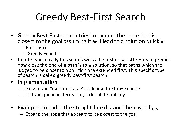
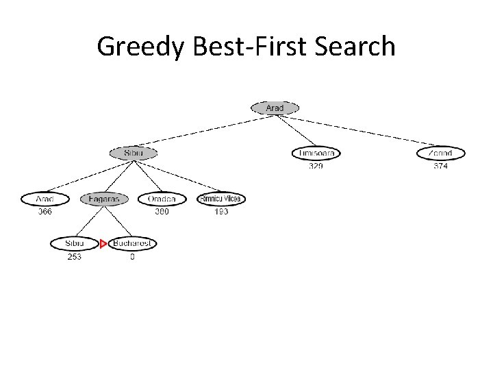
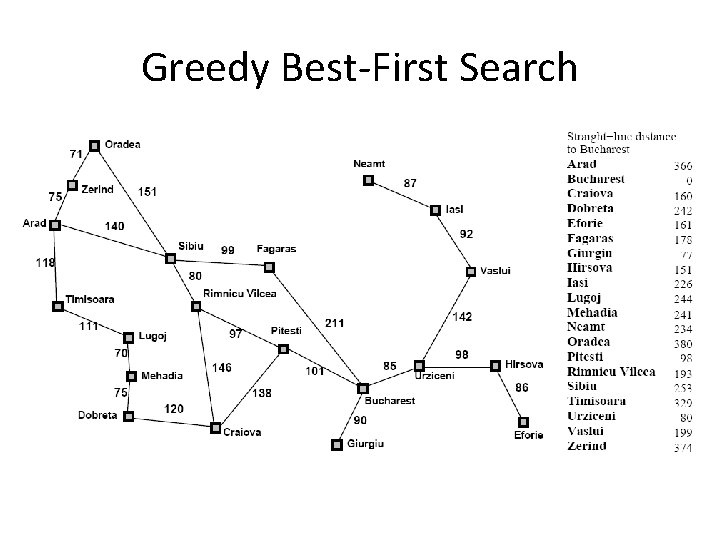
Greedy Best-First Search • Greedy Best-First search tries to expand the node that is closest to the goal assuming it will lead to a solution quickly – f(n) = h(n) – “Greedy Search” • to refer specifically to a search with a heuristic that attempts to predict how close the end of a path is to a solution, so that paths which are judged to be closer to a solution are extended first. This specific type of search is called greedy best-first search. • Implementation – expand the “most desirable” node into the fringe queue – sort the queue in decreasing order of desirability • Example: consider the straight-line distance heuristic h. SLD – Expand the node that appears to be closest to the goal

Greedy Best-First Search

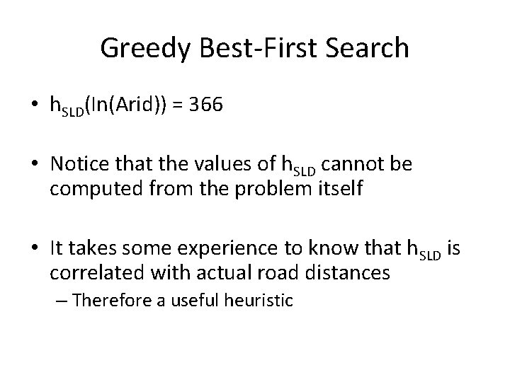
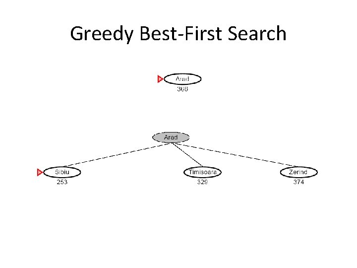
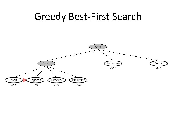
Greedy Best-First Search • h. SLD(In(Arid)) = 366 • Notice that the values of h. SLD cannot be computed from the problem itself • It takes some experience to know that h. SLD is correlated with actual road distances – Therefore a useful heuristic

Greedy Best-First Search

Greedy Best-First Search

Greedy Best-First Search

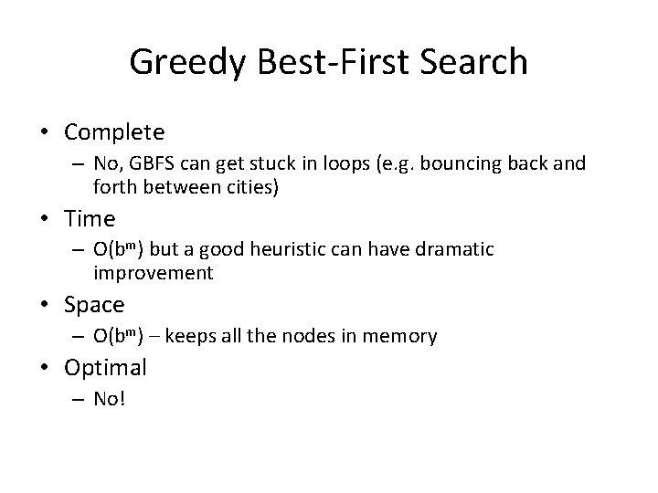
Greedy Best-First Search • Complete – No, GBFS can get stuck in loops (e. g. bouncing back and forth between cities) • Time – O(bm) but a good heuristic can have dramatic improvement • Space – O(bm) – keeps all the nodes in memory • Optimal – No!

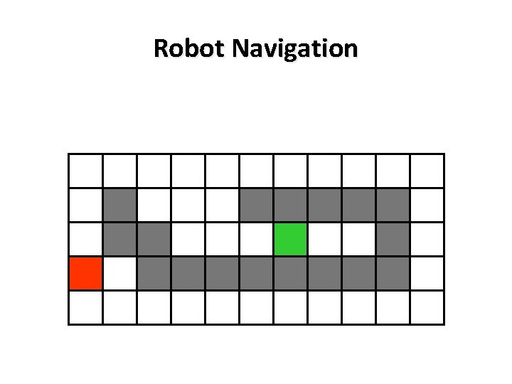
Robot Navigation

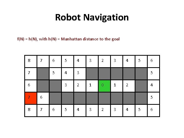
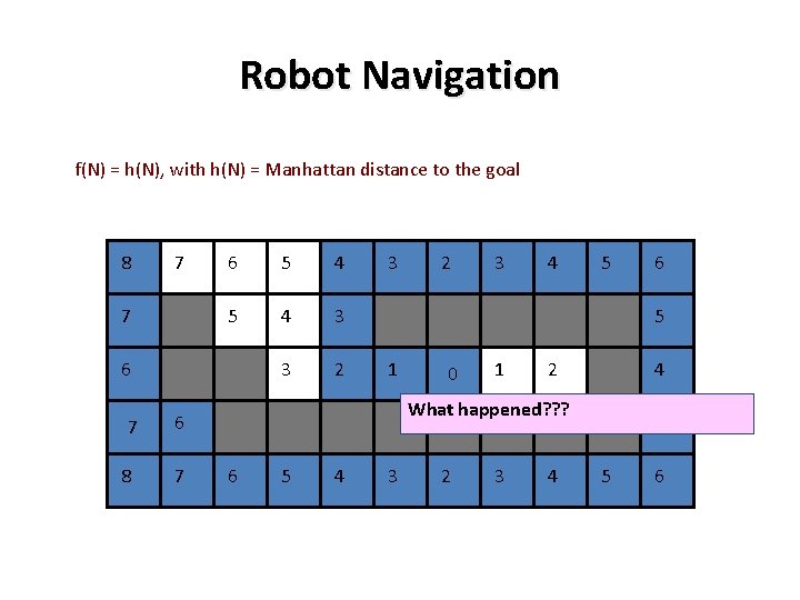
Robot Navigation f(N) = h(N), with h(N) = Manhattan distance to the goal 8 7 7 6 5 4 3 3 2 6 7 6 8 7 3 2 3 4 5 6 5 1 0 1 2 4 5 6 5 4 3 2 3 4 5 6

Robot Navigation f(N) = h(N), with h(N) = Manhattan distance to the goal 8 7 7 6 5 4 3 3 2 6 77 6 8 7 3 2 3 4 5 5 1 00 1 2 4 What happened? ? ? 6 5 4 6 3 2 3 4 5 5 6

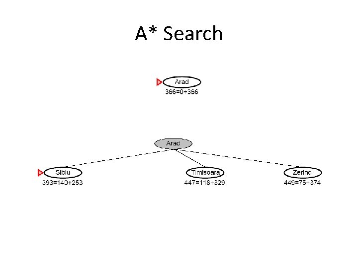
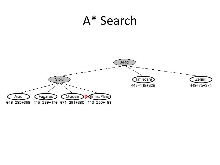
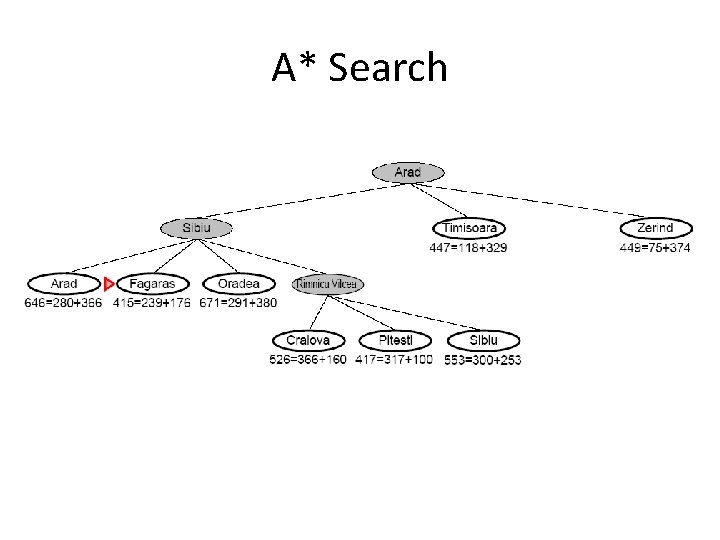
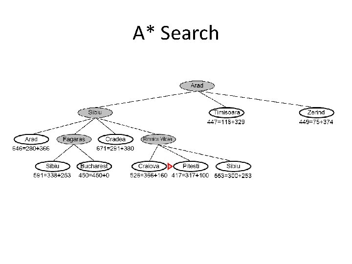
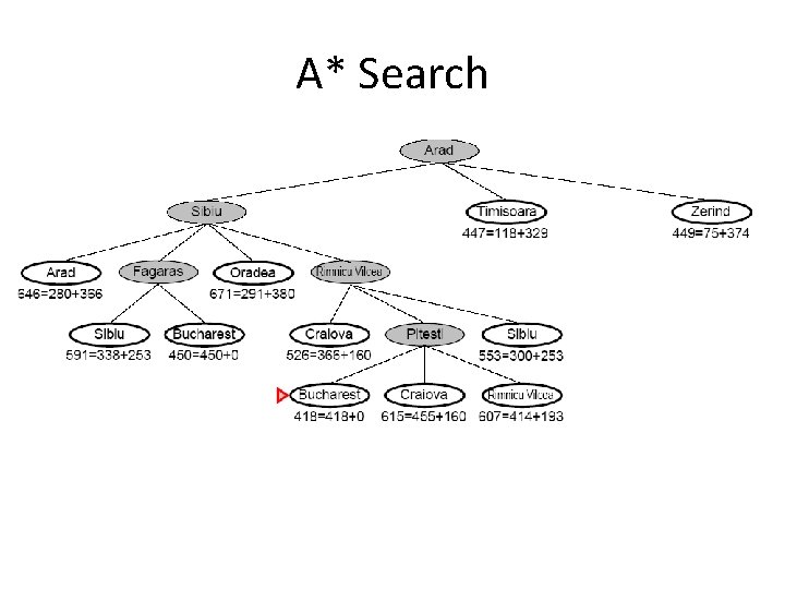
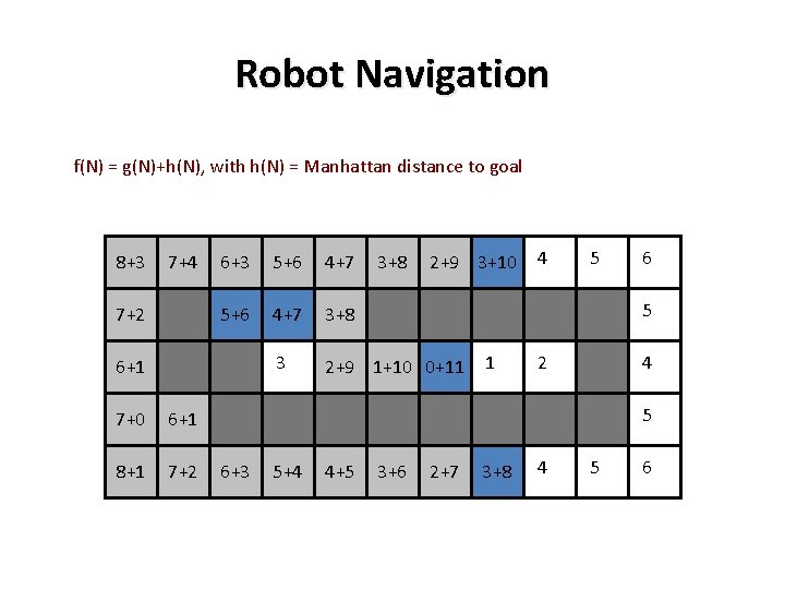
A* Search • A* algorithm is a best-first search algorithm in which the cost associated with a node is f(n) = g(n) + h(n), where g(n) is the cost of the path from the initial state to node n and h(n) is the heuristic estimate or the cost or a path from node n to a goal. • Thus, f(n) estimates the lowest total cost of any solution path going through node n. At each point a node with lowest f value is chosen for expansion. • Ties among nodes of equal f value should be broken in favor of nodes with lower h values. The algorithm terminates when a goal is chosen for expansion.

A* Search • A* (A star) is the most widely known in AI – It evaluates nodes by combining g(n) and h(n) – f(n) = g(n) + h(n) – Where • g(n) = cost so far to reach n • h(n) = estimated cost to goal from n • f(n) = estimated total cost of path through n

A* Search • When h(n) = actual cost to goal – Only nodes in the correct path are expanded – Optimal solution is found • When h(n) < actual cost to goal – Additional nodes are expanded – Optimal solution is found • When h(n) > actual cost to goal – Optimal solution can be overlooked

Greedy Best-First Search

A* Search

A* Search

A* Search

A* Search

A* Search

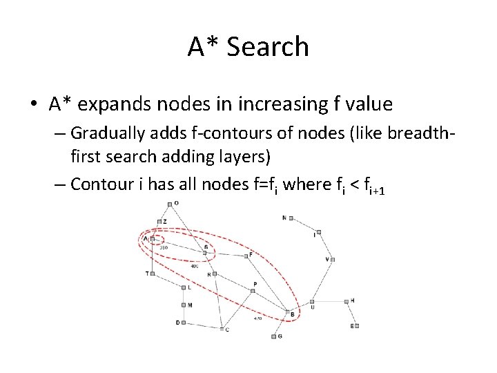
A* Search • A* expands nodes in increasing f value – Gradually adds f-contours of nodes (like breadthfirst search adding layers) – Contour i has all nodes f=fi where fi < fi+1

A* Search • Complete – Yes, unless there are infinitely many nodes with f <= f(G) • Time – Exponential in [relative error of h x length of soln] – The better the heuristic, the better the time • Best case h is perfect, O(d) • Worst case h = 0, O(bd) same as BFS • Space – Keeps all nodes in memory and save in case of repetition – This is O(bd) or worse – A* usually runs out of space before it runs out of time • Optimal – Yes, cannot expand fi+1 unless fi is finished

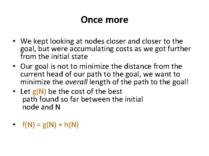
Once more • We kept looking at nodes closer and closer to the goal, but were accumulating costs as we got further from the initial state • Our goal is not to minimize the distance from the current head of our path to the goal, we want to minimize the overall length of the path to the goal! • Let g(N) be the cost of the best path found so far between the initial node and N • f(N) = g(N) + h(N)

Robot Navigation f(N) = g(N)+h(N), with h(N) = Manhattan distance to goal 8 8+3 7 7+4 7 7+2 6 6+3 6+5 5 5+6 4 4+7 3 3+8 3 2 1 0 2+9 1+10 0+11 6 6+1 7 7+0 6 6+1 8 8+1 7 7+2 3 3+8 2 3 2+9 3+10 4 5 6 5 1 2 4 5 6 6+3 5 5+4 4 4+5 3 3+6 2 2+7 3 3+8 4 5 6

Complexity Of Finding Optimal Solutions • The time complexity of a heuristic search algorithm depends on the accuracy of the heuristic function. • For example, if the heuristic evaluation function is an exact estimator, then A* search algorithm runs in linear time, expanding only those nodes on an optimal solution path. • Conversely, with a heuristic that returns zero everywhere, A* algorithm becomes uniform-cost search, which has exponential complexity.

Summery of Today’s Lecture • • Informed (Heuristic) search Heuristic evaluation function Greedy Best-First Search A* Search