S Linear Programming Models Case Studies Adapted from

S Linear Programming Models & Case Studies Adapted from lectures of Prof. Rifat Rustom 1

What is Optimization The Optimization Problem is: Find values of the variables that minimize or maximize the objective function while satisfying the constraints. 2

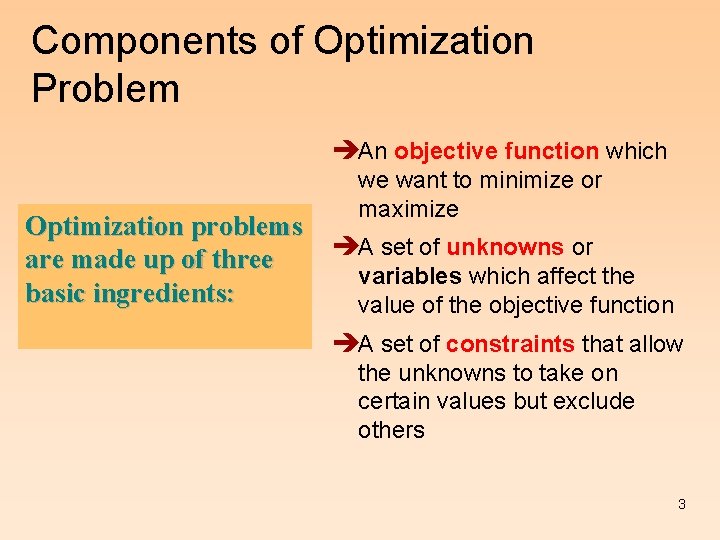
Components of Optimization Problem èAn objective function which we want to minimize or maximize Optimization problems è A set of unknowns or are made up of three variables which affect the basic ingredients: value of the objective function èA set of constraints that allow the unknowns to take on certain values but exclude others 3

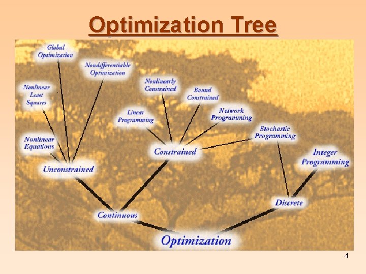
Optimization Tree 4

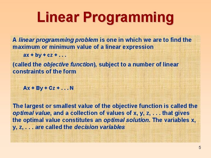
Linear Programming A linear programming problem is one in which we are to find the maximum or minimum value of a linear expression ax + by + cz +. . . (called the objective function), subject to a number of linear constraints of the form Ax + By + Cz +. . . N The largest or smallest value of the objective function is called the optimal value, and a collection of values of x, y, z, . . . that gives the optimal value constitutes an optimal solution. The variables x, y, z, . . . are called the decision variables 5

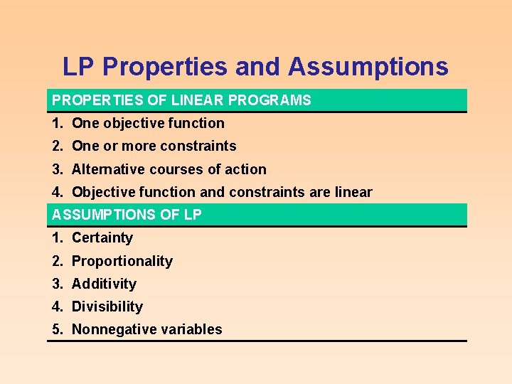
LP Properties and Assumptions PROPERTIES OF LINEAR PROGRAMS 1. One objective function 2. One or more constraints 3. Alternative courses of action 4. Objective function and constraints are linear ASSUMPTIONS OF LP 1. Certainty 2. Proportionality 3. Additivity 4. Divisibility 5. Nonnegative variables

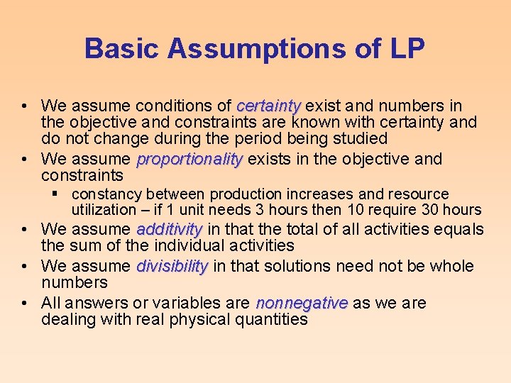
Basic Assumptions of LP • We assume conditions of certainty exist and numbers in the objective and constraints are known with certainty and do not change during the period being studied • We assume proportionality exists in the objective and constraints § constancy between production increases and resource utilization – if 1 unit needs 3 hours then 10 require 30 hours • We assume additivity in that the total of all activities equals the sum of the individual activities • We assume divisibility in that solutions need not be whole numbers • All answers or variables are nonnegative as we are dealing with real physical quantities

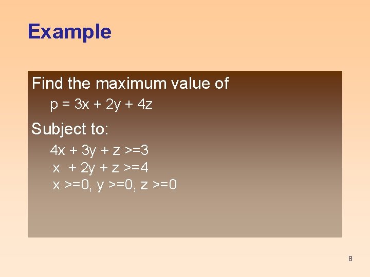
Example Find the maximum value of p = 3 x + 2 y + 4 z Subject to: 4 x + 3 y + z >=3 x + 2 y + z >=4 x >=0, y >=0, z >=0 8

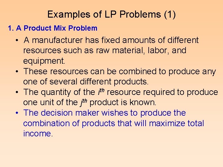
Examples of LP Problems (1) 1. A Product Mix Problem • A manufacturer has fixed amounts of different resources such as raw material, labor, and equipment. • These resources can be combined to produce any one of several different products. • The quantity of the ith resource required to produce one unit of the jth product is known. • The decision maker wishes to produce the combination of products that will maximize total income.

Examples of LP Problems (2) 2. A Blending Problem • Blending problems refer to situations in which a number of components (or commodities) are mixed together to yield one or more products. • Typically, different commodities are to be purchased. Each commodity has known characteristics and costs. • The problem is to determine how much of each commodity should be purchased and blended with the rest so that the characteristics of the mixture lie within specified bounds and the total cost is minimized.

Examples of LP Problems (3) 3. A Production Scheduling Problem • A manufacturer knows that he must supply a given number of items of a certain product each month for the next n months. • They can be produced either in regular time, subject to a maximum each month, or in overtime. The cost of producing an item during overtime is greater than during regular time. A storage cost is associated with each item not sold at the end of the month. • The problem is to determine the production schedule that minimizes the sum of production and storage costs.

Examples of LP Problems (4) 4. A Transportation Problem • A product is to be shipped in the amounts al, a 2, . . . , am from m shipping origins and received in amounts bl, b 2, . . . , bn at each of n shipping destinations. • The cost of shipping a unit from the ith origin to the jth destination is known for all combinations of origins and destinations. • The problem is to determine the amount to be shipped from each origin to each destination such that the total cost of transportation is a minimum.

Examples of LP Problems (5) 5. A Flow Capacity Problem • One or more commodities (e. g. , traffic, water, information, cash, etc. ) are flowing from one point to another through a network whose branches have various constraints and flow capacities. • The direction of flow in each branch and the capacity of each branch are known. • The problem is to determine the maximum flow, or capacity of the network.

Formulating LP Problems • Formulating a linear program involves developing a mathematical model to represent the managerial problem • The steps in formulating a linear program are 1. Completely understand the managerial problem being faced 2. Identify the objective and constraints 3. Define the decision variables 4. Use the decision variables to write mathematical expressions for the objective function and the constraints

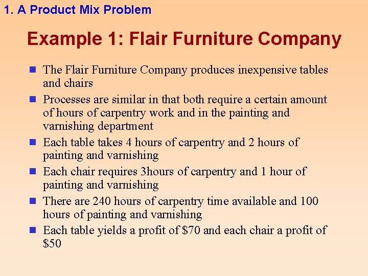
1. A Product Mix Problem Example 1: Flair Furniture Company n The Flair Furniture Company produces inexpensive tables n n n and chairs Processes are similar in that both require a certain amount of hours of carpentry work and in the painting and varnishing department Each table takes 4 hours of carpentry and 2 hours of painting and varnishing Each chair requires 3 hours of carpentry and 1 hour of painting and varnishing There are 240 hours of carpentry time available and 100 hours of painting and varnishing Each table yields a profit of $70 and each chair a profit of $50

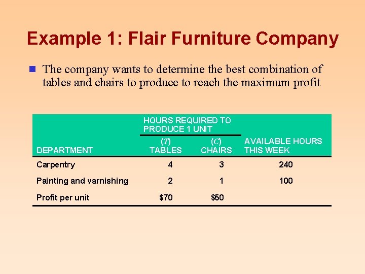
Example 1: Flair Furniture Company n The company wants to determine the best combination of tables and chairs to produce to reach the maximum profit HOURS REQUIRED TO PRODUCE 1 UNIT DEPARTMENT (T) TABLES (C) CHAIRS AVAILABLE HOURS THIS WEEK Carpentry 4 3 240 Painting and varnishing 2 1 100 $70 $50 Profit per unit

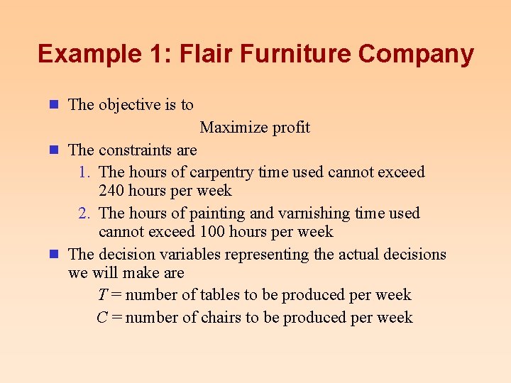
Example 1: Flair Furniture Company n The objective is to Maximize profit n The constraints are 1. The hours of carpentry time used cannot exceed 240 hours per week 2. The hours of painting and varnishing time used cannot exceed 100 hours per week n The decision variables representing the actual decisions we will make are T = number of tables to be produced per week C = number of chairs to be produced per week

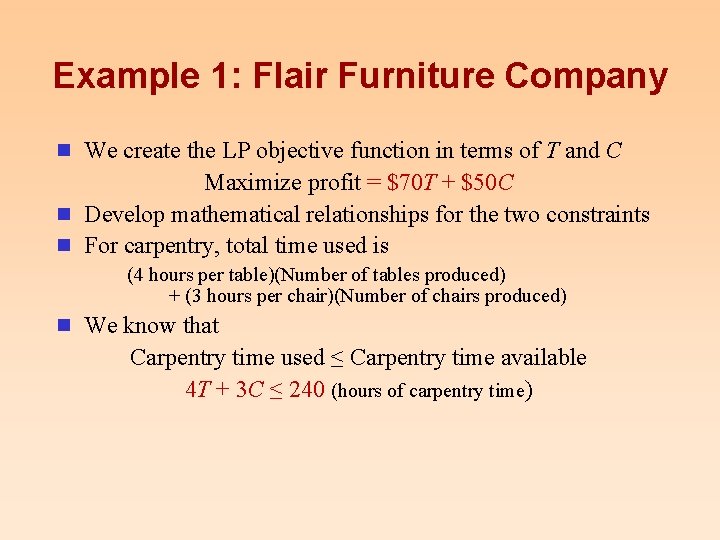
Example 1: Flair Furniture Company n We create the LP objective function in terms of T and C Maximize profit = $70 T + $50 C n Develop mathematical relationships for the two constraints n For carpentry, total time used is (4 hours per table)(Number of tables produced) + (3 hours per chair)(Number of chairs produced) n We know that Carpentry time used ≤ Carpentry time available 4 T + 3 C ≤ 240 (hours of carpentry time)

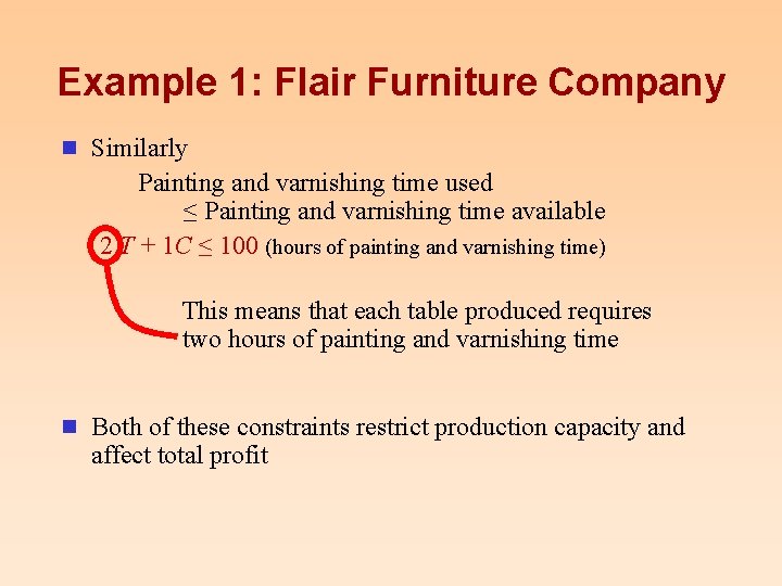
Example 1: Flair Furniture Company n Similarly Painting and varnishing time used ≤ Painting and varnishing time available 2 T + 1 C ≤ 100 (hours of painting and varnishing time) This means that each table produced requires two hours of painting and varnishing time n Both of these constraints restrict production capacity and affect total profit

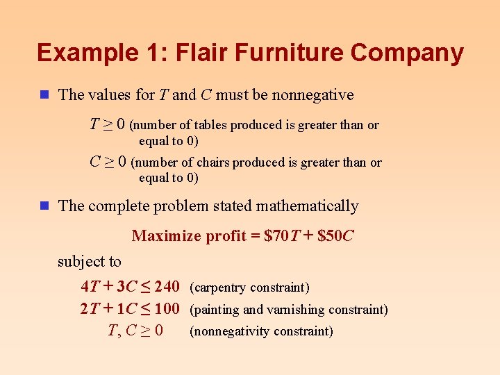
Example 1: Flair Furniture Company n The values for T and C must be nonnegative T ≥ 0 (number of tables produced is greater than or equal to 0) C ≥ 0 (number of chairs produced is greater than or equal to 0) n The complete problem stated mathematically Maximize profit = $70 T + $50 C subject to 4 T + 3 C ≤ 240 (carpentry constraint) 2 T + 1 C ≤ 100 (painting and varnishing constraint) T, C ≥ 0 (nonnegativity constraint)

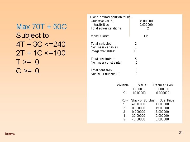
Max 70 T + 50 C Subject to 4 T + 3 C <=240 2 T + 1 C <=100 T >= 0 C >= 0 Global optimal solution found. Objective value: Infeasibilities: Total solver iterations: Model Class: LP Total variables: Nonlinear variables: Integer variables: 2 0 0 Total constraints: Nonlinear constraints: 5 0 Total nonzeros: Nonlinear nonzeros: 8 0 Variable T C Row 1 2 3 4 5 Rustom 4100. 000000 2 Value 30. 00000 40. 00000 Reduced Cost 0. 000000 Slack or Surplus 4100. 000000 30. 00000 40. 00000 Dual Price 1. 000000 15. 000000 0. 000000 21

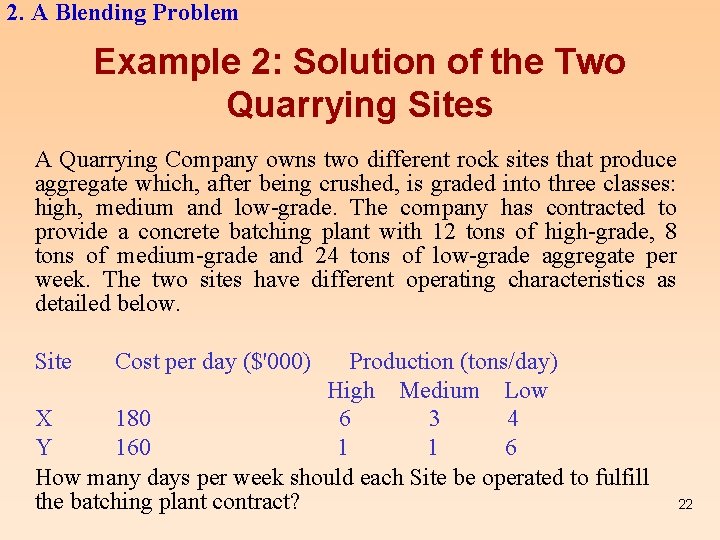
2. A Blending Problem Example 2: Solution of the Two Quarrying Sites A Quarrying Company owns two different rock sites that produce aggregate which, after being crushed, is graded into three classes: high, medium and low-grade. The company has contracted to provide a concrete batching plant with 12 tons of high-grade, 8 tons of medium-grade and 24 tons of low-grade aggregate per week. The two sites have different operating characteristics as detailed below. Site Cost per day ($'000) Production (tons/day) High Medium Low X 180 6 3 4 Y 160 1 1 6 How many days per week should each Site be operated to fulfill the batching plant contract? 22

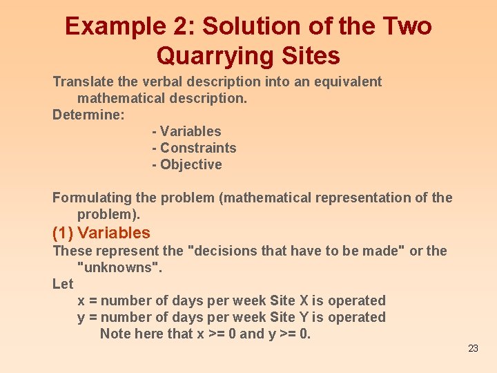
Example 2: Solution of the Two Quarrying Sites Translate the verbal description into an equivalent mathematical description. Determine: - Variables - Constraints - Objective Formulating the problem (mathematical representation of the problem). (1) Variables These represent the "decisions that have to be made" or the "unknowns". Let x = number of days per week Site X is operated y = number of days per week Site Y is operated Note here that x >= 0 and y >= 0. 23

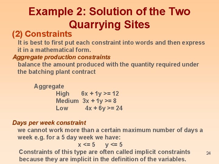
Example 2: Solution of the Two Quarrying Sites (2) Constraints It is best to first put each constraint into words and then express it in a mathematical form. Aggregate production constraints balance the amount produced with the quantity required under the batching plant contract Aggregate High 6 x + 1 y >= 12 Medium 3 x + 1 y >= 8 Low 4 x + 6 y >= 24 Days per week constraint we cannot work more than a certain maximum number of days a week e. g. for a 5 day week we have: x <= 5 y <= 5 Constraints of this type are often called implicit constraints because they are implicit in the definition of the variables. 24

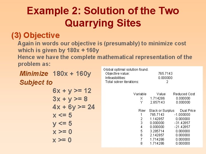
Example 2: Solution of the Two Quarrying Sites (3) Objective Again in words our objective is (presumably) to minimize cost which is given by 180 x + 160 y Hence we have the complete mathematical representation of the problem as: Minimize 180 x + 160 y Subject to 6 x + y >= 12 3 x + y >= 8 4 x + 6 y >= 24 x <= 5 y <= 5 x >= 0 Global optimal solution found. Objective value: Infeasibilities: Total solver iterations: Variable X Y Row 1 2 3 4 5 6 7 8 765. 7143 0. 000000 2 Value 1. 714286 2. 857143 Reduced Cost 0. 000000 Slack or Surplus Dual Price 765. 7143 -1. 000000 1. 142857 0. 000000 -31. 42857 0. 000000 -21. 42857 3. 285714 0. 000000 2. 142857 0. 000000 1. 714286 0. 000000 25

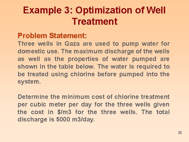
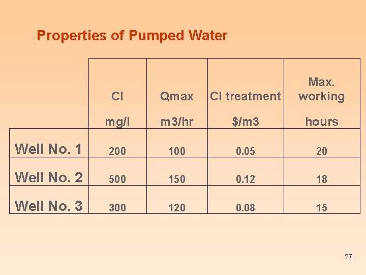
Example 3: Optimization of Well Treatment Problem Statement: Three wells in Gaza are used to pump water for domestic use. The maximum discharge of the wells as well as the properties of water pumped are shown in the table below. The water is required to be treated using chlorine before pumped into the system. Determine the minimum cost of chlorine treatment per cubic meter per day for the three wells given the cost in $/m 3 for the three wells. The total discharge is 5000 m 3/day. 26

Properties of Pumped Water Cl Qmax Cl treatment Max. working mg/l m 3/hr $/m 3 hours Well No. 1 200 100 0. 05 20 Well No. 2 500 150 0. 12 18 Well No. 3 300 120 0. 08 15 27

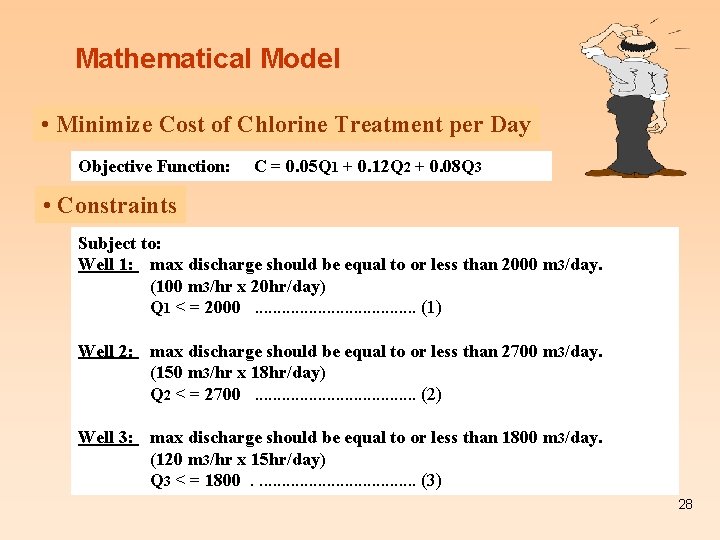
Mathematical Model • Minimize Cost of Chlorine Treatment per Day Objective Function: C = 0. 05 Q 1 + 0. 12 Q 2 + 0. 08 Q 3 • Constraints Subject to: Well 1: max discharge should be equal to or less than 2000 m 3/day. (100 m 3/hr x 20 hr/day) Q 1 < = 2000. . . . . (1) Well 2: max discharge should be equal to or less than 2700 m 3/day. (150 m 3/hr x 18 hr/day) Q 2 < = 2700. . . . . (2) Well 3: max discharge should be equal to or less than 1800 m 3/day. (120 m 3/hr x 15 hr/day) Q 3 < = 1800. . . . . (3) 28

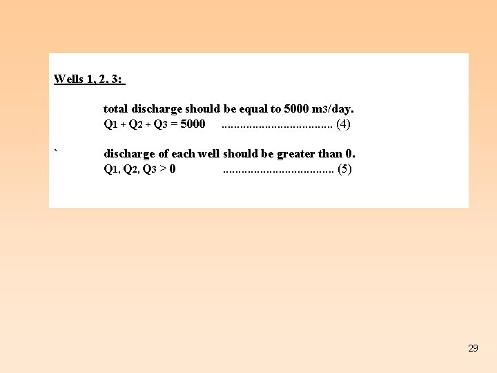
Wells 1, 2, 3: total discharge should be equal to 5000 m 3/day. Q 1 + Q 2 + Q 3 = 5000. . . . . (4) ` discharge of each well should be greater than 0. Q 1, Q 2, Q 3 > 0. . . . . (5) 29