Maplesoft Conference 2006 The Need for Formulae Manipulation

Maplesoft Conference 2006 The Need for Formulae Manipulation in the Object-oriented Modeling of Physical Systems François E. Cellier, Ph. D. Institute of Computational Science ETH Zurich Switzerland July 26, 2006 Start of Presentation

Maplesoft Conference 2006 Object-oriented Modeling • Today’s modeling needs extend to physical systems that are described by many thousands of mathematical equations. • Such models are being created and maintained by employing the principles of object-oriented graphical modeling. • Each object contains a number of different layers (aspects, realities) that are to be described shortly. • Symbolic formula manipulation plays a central role in converting these object-oriented descriptions to a form that can be simulated effectively and efficiently. Start of Presentation

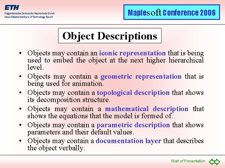
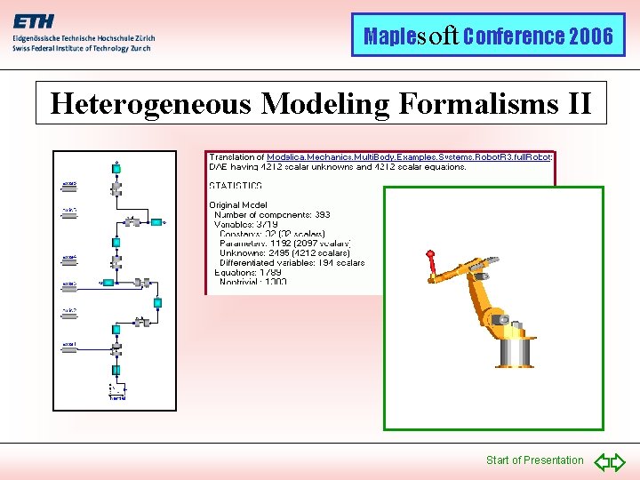
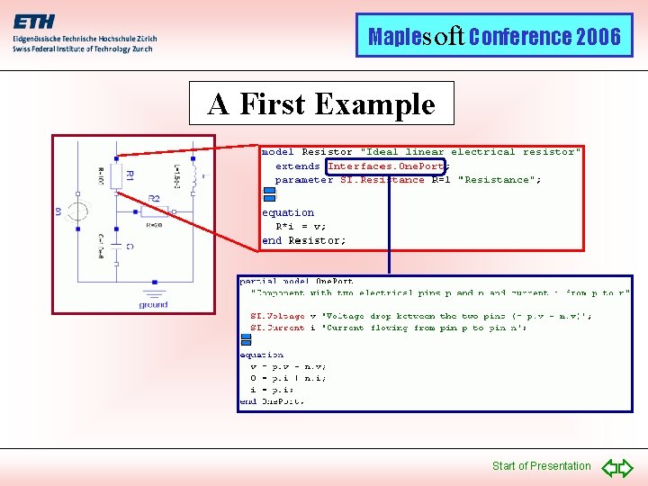
Maplesoft Conference 2006 Object Descriptions • Objects may contain an iconic representation that is being used to embed the object at the next higher hierarchical level. • Objects may contain a geometric representation that is being used for animation. • Objects may contain a topological description that shows its decomposition structure. • Objects may contain a mathematical description that shows the equations that the model is formed of. • Objects may contain a parametric description that shows parameters and their default values. • Objects may contain a documentation layer that describes the object verbally. Start of Presentation

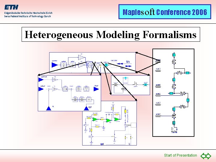
Maplesoft Conference 2006 Heterogeneous Modeling Formalisms Start of Presentation

Maplesoft Conference 2006 Heterogeneous Modeling Formalisms II Start of Presentation

Maplesoft Conference 2006 A First Example Start of Presentation

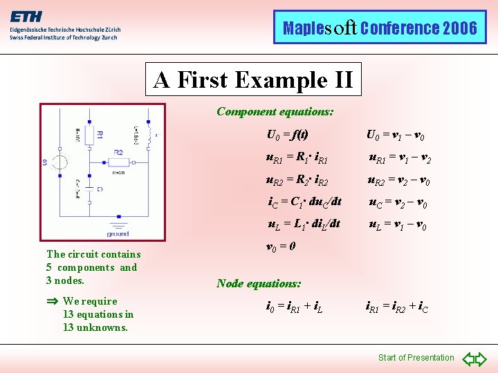
Maplesoft Conference 2006 A First Example II Component equations: The circuit contains 5 components and 3 nodes. We require 13 equations in 13 unknowns. U 0 = f(t) U 0 = v 1 – v 0 u. R 1 = R 1· i. R 1 u. R 1 = v 1 – v 2 u. R 2 = R 2· i. R 2 u. R 2 = v 2 – v 0 i. C = C 1· du. C/dt u. C = v 2 – v 0 u. L = L 1· di. L/dt u. L = v 1 – v 0 = 0 Node equations: i 0 = i. R 1 + i. L i. R 1 = i. R 2 + i. C Start of Presentation

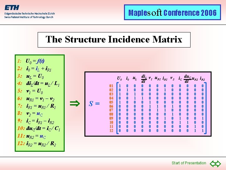
Maplesoft Conference 2006 The Structure Incidence Matrix 1: U 0 = f(t) 2: i 0 = i. L + i. R 1 3: u. L = U 0 4: di. L/dt = u. L / L 1 5: v 1 = U 0 6: u. R 1 = v 1 – v 2 7: i. R 1 = u. R 1 / R 1 8: v 2 = u. C 9: i. C = i. R 1 – i. R 2 10: du. C/dt = i. C / C 1 11: u. R 2 = u. C 12: i. R 2 = u. R 2 / R 2 U 0 S= 01 02 03 04 05 06 07 08 09 10 11 12 1 0 1 0 0 0 0 i 0 u. L 0 1 0 0 0 1 1 0 0 0 0 di. L v u i 1 R 1 v 2 dt 0 0 0 1 0 0 0 0 0 0 1 1 0 0 0 0 1 0 1 0 0 0 0 i. C du. C u. R 2 i. R 2 dt 0 0 0 0 1 1 0 0 0 0 0 0 1 1 0 0 0 0 1 Start of Presentation

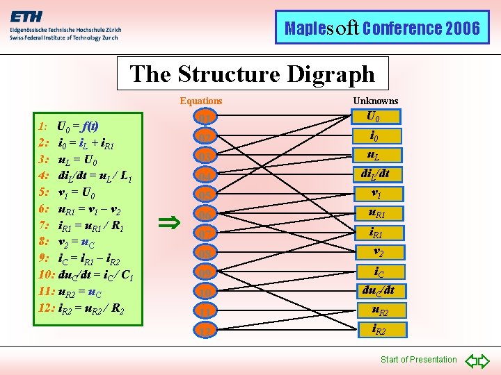
Maplesoft Conference 2006 The Structure Digraph Equations 1: U 0 = f(t) 2: i 0 = i. L + i. R 1 3: u. L = U 0 4: di. L/dt = u. L / L 1 5: v 1 = U 0 6: u. R 1 = v 1 – v 2 7: i. R 1 = u. R 1 / R 1 8: v 2 = u. C 9: i. C = i. R 1 – i. R 2 10: du. C/dt = i. C / C 1 11: u. R 2 = u. C 12: i. R 2 = u. R 2 / R 2 Unknowns 01 U 0 02 i 0 03 u. L 04 05 di. L/dt v 1 06 u. R 1 07 i. R 1 08 v 2 09 i. C 10 du. C/dt 11 u. R 2 12 i. R 2 Start of Presentation

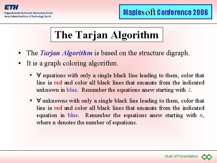
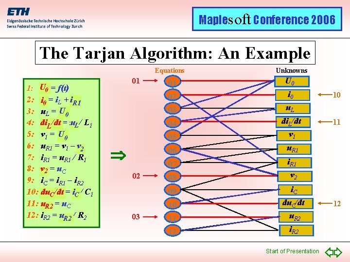
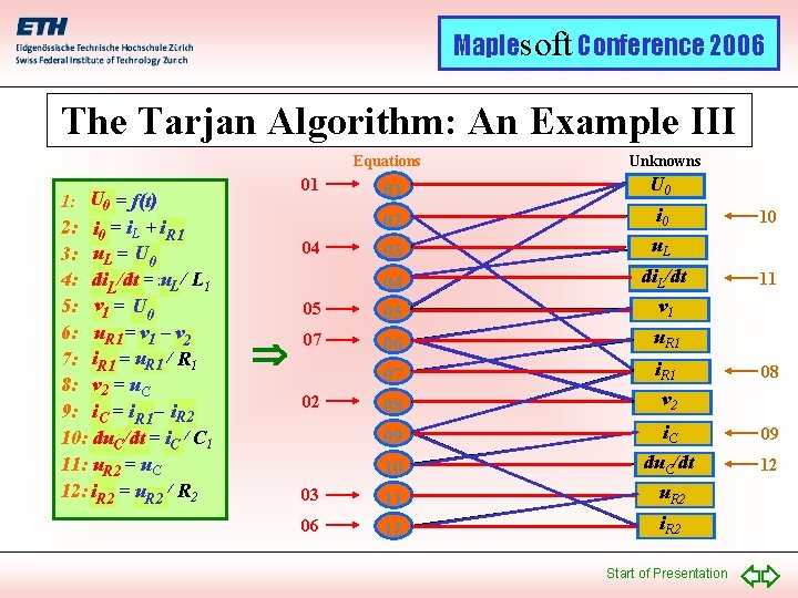
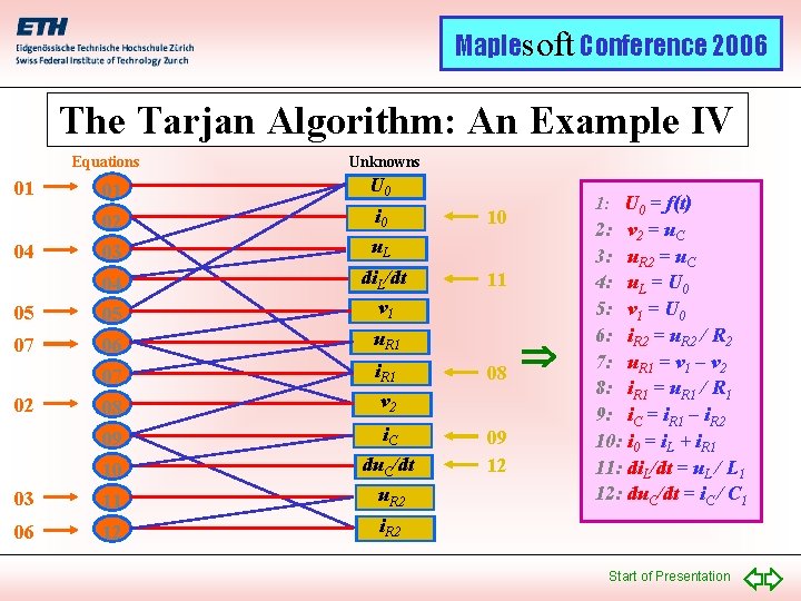
Maplesoft Conference 2006 The Tarjan Algorithm • The Tarjan Algorithm is based on the structure digraph. • It is a graph coloring algorithm. equations with only a single black line leading to them, color that line in red and color all black lines that emanate from the indicated unknown in blue. Renumber the equations anew starting with 1. unknowns with only a single black line leading to them, color that line in red and color all black lines that emanate from the indicated equation in blue. Renumber the equations anew starting with n, where n denotes the number of equations. Start of Presentation

Maplesoft Conference 2006 The Tarjan Algorithm: An Example Equations 01 1: U 00 = f(t) 2: i 0 = i. L + i. R 1 3: u. L = U 00 4: di. LL/dt = uu. L / L 1 U 00 5: v 1 = U 6: u. R 1 = v 1 – v 22 7: i. R 1 = u. R 1 / R 1 8: v 2 = u. C 9: i. C = i. R 1 – i. R 2 10: du. C/dt = i. C / C 1 11: u. R 2 = u. C 12: i. R 2 = u. R 2 / R 2 02 03 Unknowns 01 U 0 02 i 0 03 u. L 04 05 di. L/dt v 1 06 u. R 1 07 i. R 1 08 v 2 09 i. C 10 du. C/dt 11 u. R 2 12 i. R 2 Start of Presentation 10 11 12

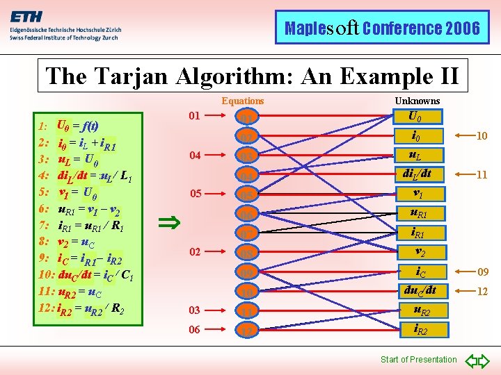
Maplesoft Conference 2006 The Tarjan Algorithm: An Example II Equations 2: i 0 = i. L + i. R 1 3: u. L = U 00 4: di. LL/dt = uu. L / L 1 U 00 5: v 1 = U 6: u. R 1 = v 11 – v 22 7: i. R 1 = u. R 1 / R 1 8: v 2 = u. C 9: i. CC = i. R 1 R 2 R 1 – i. R 2 10: du. C/dt = i. C / C 1 11: u. R 2 = u. C 12: i. R 2 = u. R 2 / R 2 01 U 0 02 i 0 03 u. L 04 05 di. L/dt v 1 06 u. R 1 07 i. R 1 08 v 2 09 i. C 09 10 du. C/dt 12 03 11 u. R 2 06 12 i. R 2 01 1: U 00 = f(t) Unknowns 04 05 02 Start of Presentation 10 11

Maplesoft Conference 2006 The Tarjan Algorithm: An Example III Equations 01 1: U 00 = f(t) 2: i 0 = i. L + i. R 1 3: u. L = U 00 4: di. LL/dt = uu. L / L 1 U 00 5: v 1 = U 6: u. R 1 = v 11 – v 22 7: i. R 1 = u. R 1 / R 1 8: v 2 = u. C 9: i. CC = i. R 1 R 2 R 1 – i. R 2 10: du. C/dt = i. C / C 1 11: u. R 2 = u. C 12: i. R 2 = u. R 2 / R 2 04 Unknowns 01 U 0 02 i 0 03 u. L 04 10 05 05 di. L/dt v 1 07 06 u. R 1 07 i. R 1 08 v 2 09 i. C 09 10 du. C/dt 12 03 11 u. R 2 06 12 i. R 2 02 Start of Presentation 11 08

Maplesoft Conference 2006 The Tarjan Algorithm: An Example IV Equations 01 04 Unknowns 01 U 0 02 i 0 03 u. L 04 05 05 di. L/dt v 1 07 06 u. R 1 07 i. R 1 08 v 2 09 i. C 10 du. C/dt 03 11 u. R 2 06 12 i. R 2 02 1: U 0 = f(t) 10 11 08 09 12 2: v 2 = u. C 3: u. R 2 = u. C 4: u. L = U 0 5: v 1 = U 0 6: i. R 2 = u. R 2 / R 2 7: u. R 1 = v 1 – v 2 8: i. R 1 = u. R 1 / R 1 9: i. C = i. R 1 – i. R 2 10: i 0 = i. L + i. R 1 11: di. L/dt = u. L / L 1 12: du. C/dt = i. C / C 1 Start of Presentation

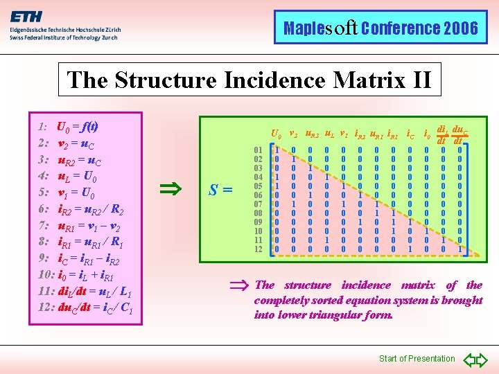
Maplesoft Conference 2006 The Structure Incidence Matrix II 1: U 0 = f(t) 2: v 2 = u. C 3: u. R 2 = u. C 4: u. L = U 0 5: v 1 = U 0 6: i. R 2 = u. R 2 / R 2 7: u. R 1 = v 1 – v 2 8: i. R 1 = u. R 1 / R 1 9: i. C = i. R 1 – i. R 2 10: i 0 = i. L + i. R 1 11: di. L/dt = u. L / L 1 12: du. C/dt = i. C / C 1 U 0 v 2 u. R 2 u. L v 1 i. R 2 u. R 1 i. C S= 01 02 03 04 05 06 07 08 09 10 11 12 1 0 0 1 1 0 0 0 0 0 0 0 1 0 0 0 0 0 1 0 0 0 0 0 1 1 0 0 0 1 1 1 0 0 0 0 0 1 i 0 di. L du. C dt dt 0 0 0 0 0 1 0 The 0 0 0 1 structure incidence matrix of the completely sorted equation system is brought into lower triangular form. Start of Presentation

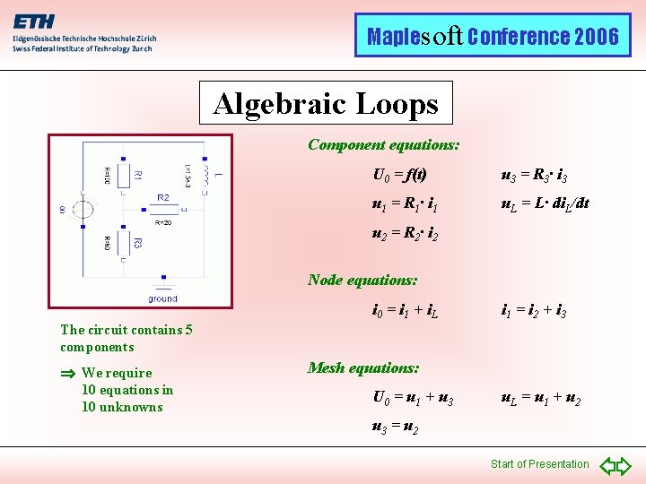
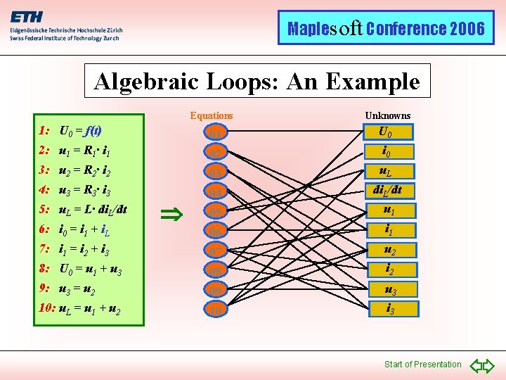
Maplesoft Conference 2006 Algebraic Loops Component equations: U 0 = f(t) u 3 = R 3 · i 3 u 1 = R 1 · i 1 u. L = L· di. L/dt u 2 = R 2 · i 2 Node equations: i 0 = i 1 + i. L i 1 = i 2 + i 3 The circuit contains 5 components We require 10 equations in 10 unknowns Mesh equations: U 0 = u 1 + u 3 u. L = u 1 + u 2 u 3 = u 2 Start of Presentation

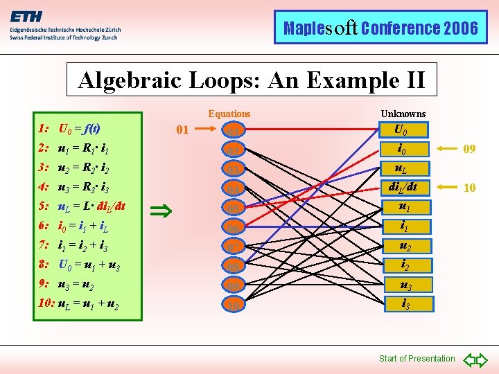
Maplesoft Conference 2006 Algebraic Loops: An Example Equations Unknowns 1: U 0 = f(t) 01 U 0 2: u 1 = R 1· i 1 02 i 0 3: u 2 = R 2· i 2 03 u. L 4: u 3 = R 3· i 3 04 05 di. L/dt u 1 06 i 1 7: i 1 = i 2 + i 3 07 u 2 8: U 0 = u 1 + u 3 08 i 2 9: u 3 = u 2 09 u 3 10: u. L = u 1 + u 2 10 i 3 5: u. L = L· di. L/dt 6: i 0 = i 1 + i. L Start of Presentation

Maplesoft Conference 2006 Algebraic Loops: An Example II Equations 1: U 0 = f(t) Unknowns 01 U 0 2: u 1 = R 1· i 1 02 i 0 3: u 2 = R 2· i 2 03 u. L 4: u 3 = R 3· i 3 04 05 di. L/dt u 1 06 i 1 7: i 1 = i 2 + i 3 07 u 2 8: U 0 = u 1 + u 3 08 i 2 9: u 3 = u 2 09 u 3 10: u. L = u 1 + u 2 10 i 3 5: u. L = L· di. L/dt 6: i 0 = i 1 + i. L 01 Start of Presentation 09 10

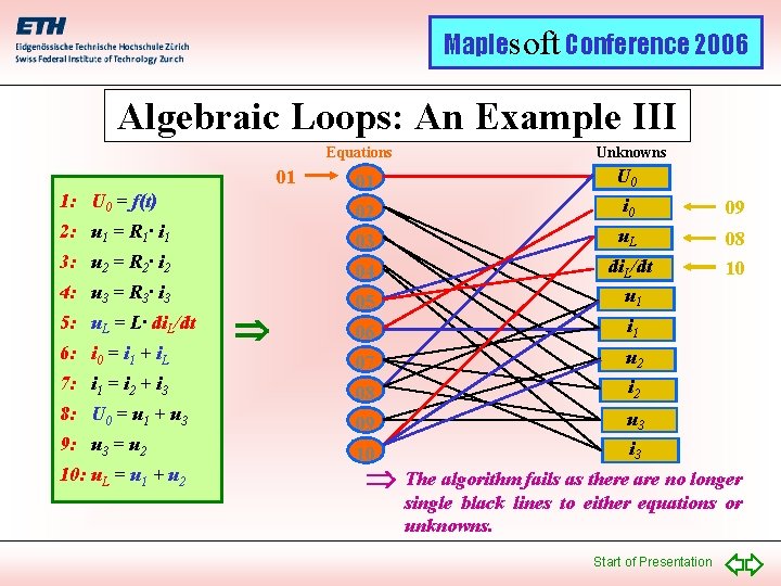
Maplesoft Conference 2006 Algebraic Loops: An Example III Equations 01 1: U 0 = f(t) 2: u 1 = R 1· i 1 3: u 2 = R 2· i 2 4: u 3 = R 3· i 3 5: u. L = L· di. L/dt 6: i 0 = i 1 + i. L 7: i 1 = i 2 + i 3 8: U 0 = u 1 + u 3 9: u 3 = u 2 10: u. L = u 1 + u 2 Unknowns 01 U 0 02 i 0 09 03 u. L 04 05 di. L/dt u 1 08 10 06 i 1 07 u 2 08 i 2 09 u 3 10 i 3 The algorithm fails as there are no longer single black lines to either equations or unknowns. Start of Presentation

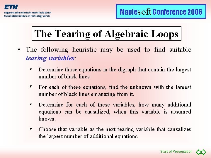
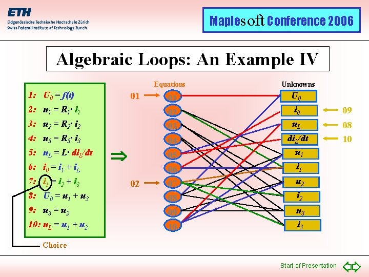
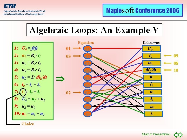
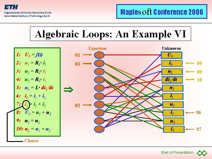
Maplesoft Conference 2006 The Tearing of Algebraic Loops • The following heuristic may be used to find suitable tearing variables: Determine those equations in the digraph that contain the largest number of black lines. For each of these equations, find the unknown with the largest number of black lines emanating from it. Determine for each of these variables, how many additional equations can be causalized, when this variable is assumed known. Choose that variable as the next tearing variable that causalizes the largest number of additional equations. Start of Presentation

Maplesoft Conference 2006 Algebraic Loops: An Example IV Equations 1: U 0 = f(t) Unknowns 01 U 0 2: u 1 = R 1· i 1 02 i 0 09 3: u 2 = R 2· i 2 03 u. L 4: u 3 = R 3· i 3 04 05 di. L/dt u 1 08 10 06 i 1 07 u 2 8: U 0 = u 1 + u 3 08 i 2 9: u 3 = u 2 09 u 3 10: u. L = u 1 + u 2 10 i 3 5: u. L = L· di. L/dt 6: i 0 = i 1 + i. L 7: i 1 = i 2 + i 3 01 02 Choice Start of Presentation

Maplesoft Conference 2006 Algebraic Loops: An Example V Equations Unknowns 1: U 0 = f(t) 01 01 U 0 2: u 1 = R 1· i 1 03 02 i 0 09 3: u 2 = R 2· i 2 03 u. L 4: u 3 = R 3· i 3 04 05 di. L/dt u 1 08 10 06 i 1 07 u 2 8: U 0 = u 1 + u 3 08 i 2 9: u 3 = u 2 09 u 3 10: u. L = u 1 + u 2 10 i 3 5: u. L = L· di. L/dt 6: i 0 = i 1 + i. L 7: i 1 = i 2 + i 3 02 Choice Start of Presentation

Maplesoft Conference 2006 Algebraic Loops: An Example VI Equations Unknowns 1: U 0 = f(t) 01 01 U 0 2: u 1 = R 1· i 1 03 02 i 0 09 3: u 2 = R 2· i 2 03 u. L 4: u 3 = R 3· i 3 04 05 di. L/dt u 1 08 10 06 i 1 07 u 2 8: U 0 = u 1 + u 3 08 i 2 9: u 3 = u 2 09 u 3 10: u. L = u 1 + u 2 10 i 3 5: u. L = L· di. L/dt 6: i 0 = i 1 + i. L 7: i 1 = i 2 + i 3 02 Choice Start of Presentation 06 07

Maplesoft Conference 2006 Algebraic Loops: An Example VII Equations Unknowns 1: U 0 = f(t) 01 01 U 0 2: u 1 = R 1· i 1 03 02 i 0 09 3: u 2 = R 2· i 2 03 u. L 4: u 3 = R 3· i 3 04 05 di. L/dt u 1 08 10 06 i 1 5: u. L = L· di. L/dt 6: i 0 = i 1 + i. L 7: i 1 = i 2 + i 3 02 07 u 2 8: U 0 = u 1 + u 3 04 08 i 2 9: u 3 = u 2 09 u 3 10: u. L = u 1 + u 2 10 i 3 Choice Start of Presentation 06 07

Maplesoft Conference 2006 Algebraic Loops: An Example VIII Equations Unknowns 1: U 0 = f(t) 01 01 U 0 2: u 1 = R 1· i 1 03 02 i 0 09 3: u 2 = R 2· i 2 03 u. L 4: u 3 = R 3· i 3 04 05 di. L/dt u 1 08 10 06 i 1 5: u. L = L· di. L/dt 6: i 0 = i 1 + i. L 7: i 1 = i 2 + i 3 02 07 u 2 05 8: U 0 = u 1 + u 3 04 08 i 2 06 9: u 3 = u 2 09 u 3 10: u. L = u 1 + u 2 10 i 3 Choice Start of Presentation 07

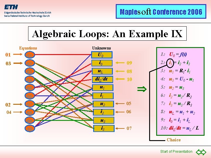
Maplesoft Conference 2006 Algebraic Loops: An Example IX Equations Unknowns 1: U 0 = f(t) 01 01 U 0 03 02 i 0 09 2: i 1 = i 2 + i 3 03 u. L 3: u 1 = R 1· i 1 04 05 di. L/dt u 1 08 10 06 i 1 02 07 u 2 05 7: i 3 = u 3 / R 3 04 08 i 2 06 8: u. L = u 1 + u 2 09 u 3 10 i 3 4: u 3 = U 0 - u 1 5: u 2 = u 3 6: i 2 = u 2 / R 2 9: i 0 = i 1 + i. L 07 10: di. L/dt = u. L / L Choice Start of Presentation

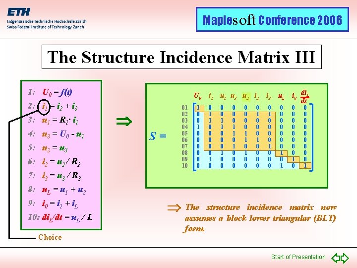
Maplesoft Conference 2006 The Structure Incidence Matrix III 1: U 0 = f(t) 2: i 1 = i 2 + i 3 3: u 1 = R 1· i 1 4: u 3 = U 0 - u 1 5: u 2 = u 3 6: i 2 = u 2 / R 2 U 0 S= 01 02 03 04 05 06 07 08 09 10 1 0 0 0 0 i 1 u 3 ui 22 i 2 0 1 1 0 0 0 1 0 0 0 0 0 1 1 0 1 0 0 0 0 i 3 u. L 0 1 0 0 0 0 1 i 0 di. L dt 0 0 0 0 1 0 0 0 0 0 1 7: i 3 = u 3 / R 3 8: u. L = u 1 + u 2 9: i 0 = i 1 + i. L 10: di. L/dt = u. L / L Choice The structure incidence matrix now assumes a block lower triangular (BLT) form. Start of Presentation

Maplesoft Conference 2006 The Solving of Algebraic Loops I • The Tarjan algorithm identifies and isolates algebraic loops. • It transforms the structure incidence matrix to BLT form, whereby the diagonal blocks are made as small as possible. • The selection of the tearing variables is not done in a truly optimal fashion. This is not meaningful, because the optimal selection of tearing variables has been shown to be an np-complete problem. Instead, a set of heuristics is being used, which usually comes up with a small number of tearing variables, although the number may not be truly minimal. • The Tarjan algorithm does not concern itself with how the resulting algebraic loops are being solved. Start of Presentation

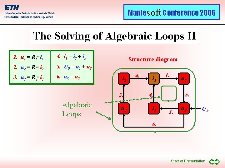
Maplesoft Conference 2006 The Solving of Algebraic Loops II 1. u 1 = R 1· i 1 4. i 1 = i 2 + i 3 2. u 2 = R 2· i 2 5. U 0 = u 1 + u 3 3. u 3 = R 3· i 3 6. u 3 = u 2 Structure diagram i 2 2. Algebraic Loops u 2 4. i 1 1. u 1 5. 4. i 3 3. u 3 U 0 6. Start of Presentation

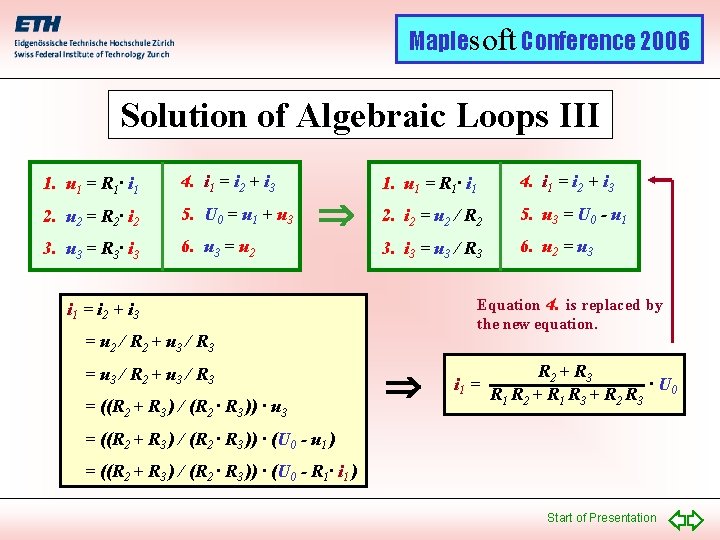
Maplesoft Conference 2006 Solution of Algebraic Loops III 1. u 1 = R 1· i 1 4. i 1 = i 2 + i 3 2. u 2 = R 2· i 2 5. U 0 = u 1 + u 3 3. u 3 = R 3· i 3 6. u 3 = u 2 1. u 1 = R 1· i 1 4. i 1 = i 2 + i 3 2. i 2 = u 2 / R 2 5. u 3 = U 0 - u 1 3. i 3 = u 3 / R 3 6. u 2 = u 3 Equation 4. is replaced by the new equation. i 1 = i 2 + i 3 = u 2 / R 2 + u 3 / R 3 = u 3 / R 2 + u 3 / R 3 = ((R 2 + R 3 ) / (R 2 · R 3 )) · u 3 i 1 = R 2 + R 3 · U 0 R 1 R 2 + R 1 R 3 + R 2 R 3 = ((R 2 + R 3 ) / (R 2 · R 3 )) · (U 0 - u 1 ) = ((R 2 + R 3 ) / (R 2 · R 3 )) · (U 0 - R 1· i 1 ) Start of Presentation

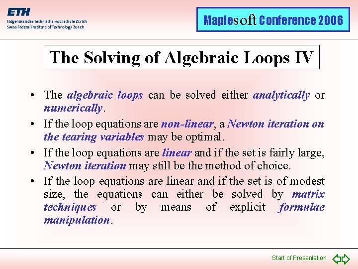
Maplesoft Conference 2006 The Solving of Algebraic Loops IV • The algebraic loops can be solved either analytically or numerically. • If the loop equations are non-linear, a Newton iteration on the tearing variables may be optimal. • If the loop equations are linear and if the set is fairly large, Newton iteration may still be the method of choice. • If the loop equations are linear and if the set is of modest size, the equations can either be solved by matrix techniques or by means of explicit formulae manipulation. Start of Presentation

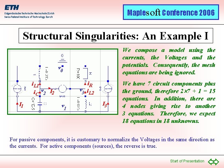
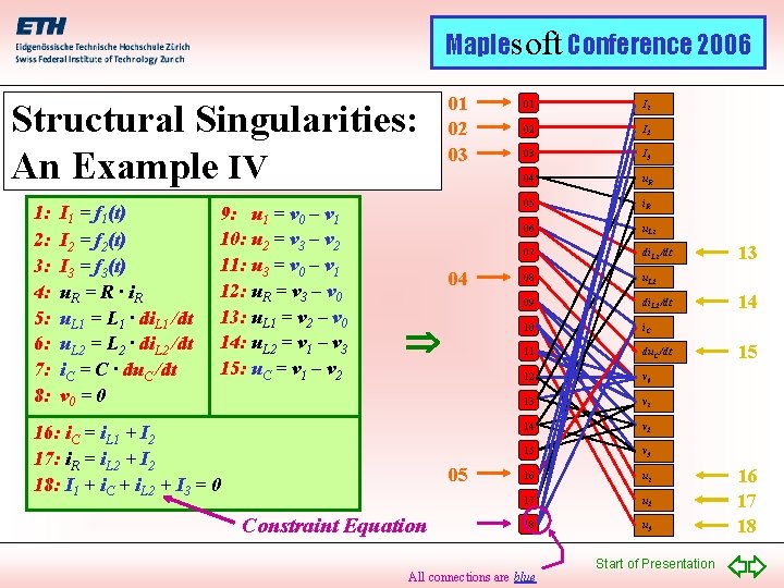
Maplesoft Conference 2006 Structural Singularities: An Example I We compose a model using the currents, the Voltages and the potentials. Consequently, the mesh equations are being ignored. v 0 i. R v 3 i L 2 i. L 1 i. C v 2 I 1 v 1 I 3 We have 7 circuit components plus the ground, therefore 2 7 + 1 = 15 equations. In addition, there are 4 nodes giving rise to another 3 equations. Therefore, we expect 18 equations in 18 unknowns. For passive components, it is customary to normalize the Voltages in the same direction as the currents. For active components (sources), the reverse is true. Start of Presentation

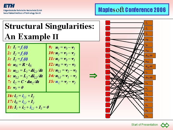
Maplesoft Conference 2006 Structural Singularities: An Example II 1: 2: 3: 4: 5: 6: 7: 8: I 1 = f 1(t) I 2 = f 2(t) I 3 = f 3(t) u. R = R · i R u. L 1 = L 1 · di. L 1 /dt u. L 2 = L 2 · di. L 2 /dt i. C = C · du. C /dt v 0 = 0 9: u 1 = v 0 – v 1 10: u 2 = v 3 – v 2 11: u 3 = v 0 – v 1 12: u. R = v 3 – v 0 13: u. L 1 = v 2 – v 0 14: u. L 2 = v 1 – v 3 15: u. C = v 1 – v 2 16: i. C = i. L 1 + I 2 17: i. R = i. L 2 + I 2 18: I 1 + i. C + i. L 2 + I 3 = 0 01 I 1 02 I 2 03 I 3 04 u. R 05 i. R 06 u. L 1 07 di. L 1 /dt 08 u. L 2 09 di. L 2 /dt 10 i. C 11 du. C /dt 12 v 0 13 v 1 14 v 2 15 v 3 16 u 1 17 u 2 18 u 3 Start of Presentation

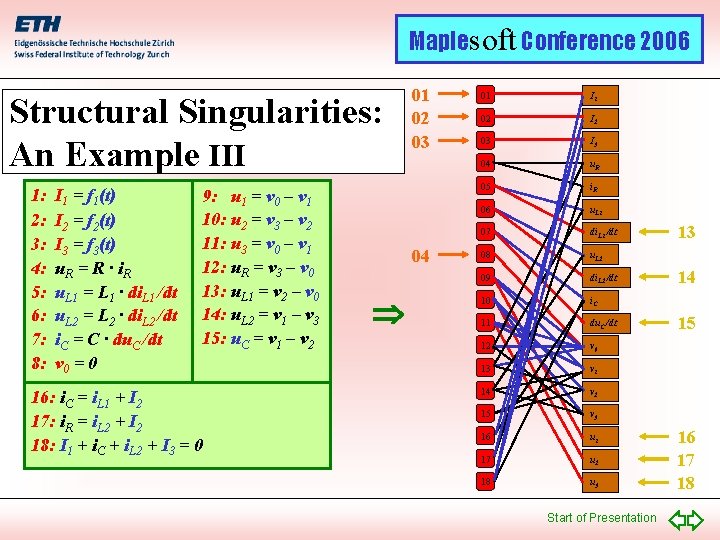
Maplesoft Conference 2006 Structural Singularities: An Example III 1: 2: 3: 4: 5: 6: 7: 8: I 1 = f 1(t) I 2 = f 2(t) I 3 = f 3(t) u. R = R · i R u. L 1 = L 1 · di. L 1 /dt u. L 2 = L 2 · di. L 2 /dt i. C = C · du. C /dt v 0 = 0 9: u 1 = v 0 – v 1 10: u 2 = v 3 – v 2 11: u 3 = v 0 – v 1 12: u. R = v 3 – v 0 13: u. L 1 = v 2 – v 0 14: u. L 2 = v 1 – v 3 15: u. C = v 1 – v 2 16: i. C = i. L 1 + I 2 17: i. R = i. L 2 + I 2 18: I 1 + i. C + i. L 2 + I 3 = 0 01 02 03 04 01 I 1 02 I 2 03 I 3 04 u. R 05 i. R 06 u. L 1 07 di. L 1 /dt 08 u. L 2 09 di. L 2 /dt 10 i. C 11 du. C /dt 12 v 0 13 v 1 14 v 2 15 v 3 16 u 1 17 u 2 18 u 3 Start of Presentation 13 14 15 16 17 18

Maplesoft Conference 2006 Structural Singularities: An Example IV 1: 2: 3: 4: 5: 6: 7: 8: I 1 = f 1(t) I 2 = f 2(t) I 3 = f 3(t) u. R = R · i R u. L 1 = L 1 · di. L 1 /dt u. L 2 = L 2 · di. L 2 /dt i. C = C · du. C /dt v 0 = 0 9: u 1 = v 0 – v 1 10: u 2 = v 3 – v 2 11: u 3 = v 0 – v 1 12: u. R = v 3 – v 0 13: u. L 1 = v 2 – v 0 14: u. L 2 = v 1 – v 3 15: u. C = v 1 – v 2 01 02 03 04 16: i. C = i. L 1 + I 2 17: i. R = i. L 2 + I 2 18: I 1 + i. C + i. L 2 + I 3 = 0 05 Constraint Equation 01 I 1 02 I 2 03 I 3 04 u. R 05 i. R 06 u. L 1 07 di. L 1 /dt 08 u. L 2 09 di. L 2 /dt 10 i. C 11 du. C /dt 12 v 0 13 v 1 14 v 2 15 v 3 16 u 1 17 u 2 18 u 3 All connections are blue Start of Presentation 13 14 15 16 17 18

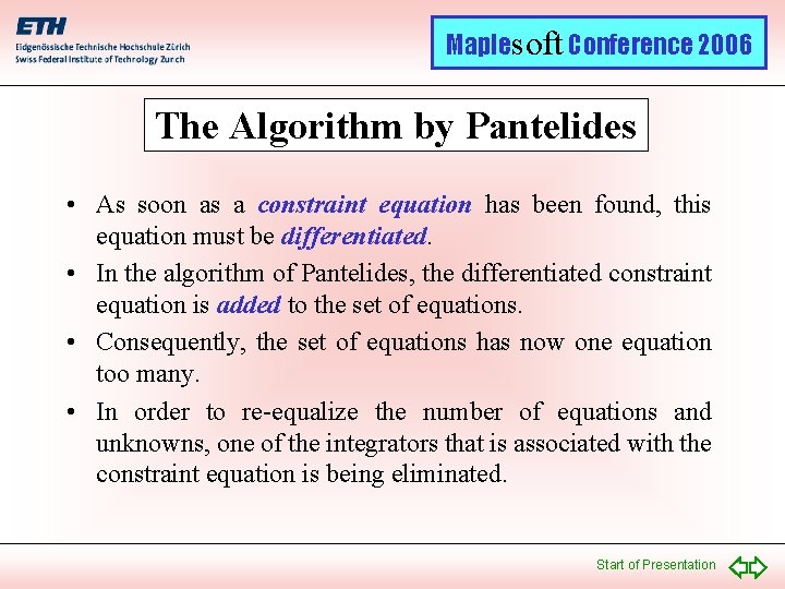
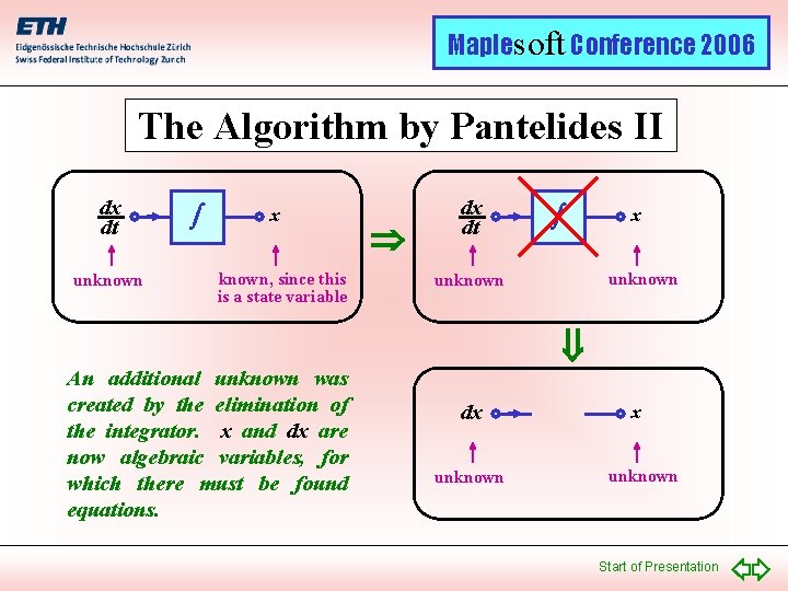
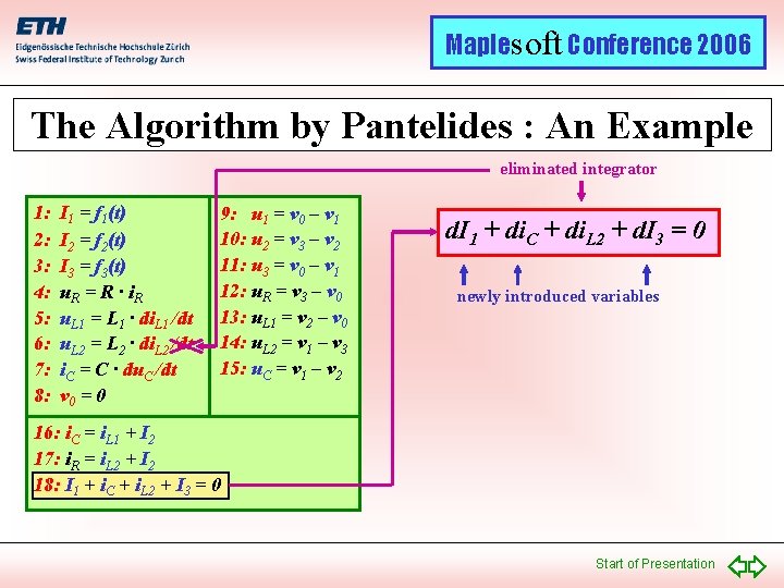
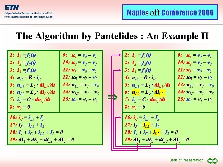
Maplesoft Conference 2006 The Algorithm by Pantelides • As soon as a constraint equation has been found, this equation must be differentiated. • In the algorithm of Pantelides, the differentiated constraint equation is added to the set of equations. • Consequently, the set of equations has now one equation too many. • In order to re-equalize the number of equations and unknowns, one of the integrators that is associated with the constraint equation is being eliminated. Start of Presentation

Maplesoft Conference 2006 The Algorithm by Pantelides II dx dt unknown x known, since this is a state variable dx dt x unknown An additional unknown was created by the elimination of the integrator. x and dx are now algebraic variables, for which there must be found equations. dx unknown Start of Presentation

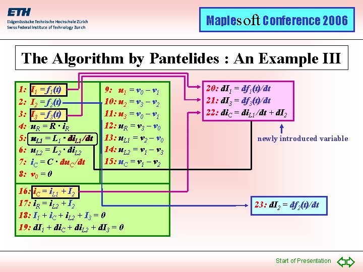
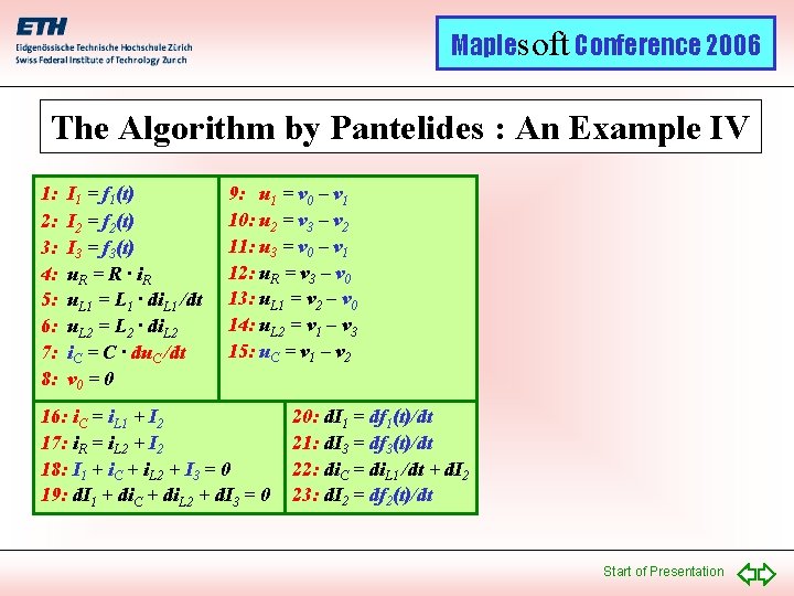
Maplesoft Conference 2006 The Algorithm by Pantelides III • When differentiating constraint equations, it can happen that additional new variables are being created, e. g. v dv, where v is an algebraic variable. • Since v was already blue (otherwise, this would not have been a constraint equation), there already exists another equation to compute v. • This equation must also be differentiated. • The differentiation of additional equations continues until no additional variables are being created. Start of Presentation

Maplesoft Conference 2006 The Algorithm by Pantelides : An Example eliminated integrator 1: 2: 3: 4: 5: 6: 7: 8: I 1 = f 1(t) I 2 = f 2(t) I 3 = f 3(t) u. R = R · i R u. L 1 = L 1 · di. L 1 /dt u. L 2 = L 2 · di. L 2 /dt i. C = C · du. C /dt v 0 = 0 9: u 1 = v 0 – v 1 10: u 2 = v 3 – v 2 11: u 3 = v 0 – v 1 12: u. R = v 3 – v 0 13: u. L 1 = v 2 – v 0 14: u. L 2 = v 1 – v 3 15: u. C = v 1 – v 2 d. I 1 + di. C + di. L 2 + d. I 3 = 0 newly introduced variables 16: i. C = i. L 1 + I 2 17: i. R = i. L 2 + I 2 18: I 1 + i. C + i. L 2 + I 3 = 0 Start of Presentation

Maplesoft Conference 2006 The Algorithm by Pantelides : An Example II 1: 2: 3: 4: 5: 6: 7: 8: I 1 = f 1(t) I 2 = f 2(t) I 3 = f 3(t) u. R = R · i R u. L 1 = L 1 · di. L 1 /dt u. L 2 = L 2 · di. L 2 /dt i. C = C · du. C /dt v 0 = 0 9: u 1 = v 0 – v 1 10: u 2 = v 3 – v 2 11: u 3 = v 0 – v 1 12: u. R = v 3 – v 0 13: u. L 1 = v 2 – v 0 14: u. L 2 = v 1 – v 3 15: u. C = v 1 – v 2 16: i. C = i. L 1 + I 2 17: i. R = i. L 2 + I 2 18: I 1 + i. C + i. L 2 + I 3 = 0 19: d. I 1 + di. C + di. L 2 + d. I 3 = 0 1: 2: 3: 4: 5: 6: 7: 8: I 1 = f 1(t) I 2 = f 2(t) I 3 = f 3(t) u. R = R · i R u. L 1 = L 1 · di. L 1 /dt u. L 2 = L 2 · di. L 2 i. C = C · du. C /dt v 0 = 0 9: u 1 = v 0 – v 1 10: u 2 = v 3 – v 2 11: u 3 = v 0 – v 1 12: u. R = v 3 – v 0 13: u. L 1 = v 2 – v 0 14: u. L 2 = v 1 – v 3 15: u. C = v 1 – v 2 16: i. C = i. L 1 + I 2 17: i. R = i. L 2 + I 2 18: I 1 + i. C + i. L 2 + I 3 = 0 19: d. I 1 + di. C + di. L 2 + d. I 3 = 0 Start of Presentation

Maplesoft Conference 2006 The Algorithm by Pantelides : An Example III 1: 2: 3: 4: 5: 6: 7: 8: I 1 = f 1(t) I 2 = f 2(t) I 3 = f 3(t) u. R = R · i R u. L 1 = L 1 · di. L 1 /dt u. L 2 = L 2 · di. L 2 i. C = C · du. C /dt v 0 = 0 9: u 1 = v 0 – v 1 10: u 2 = v 3 – v 2 11: u 3 = v 0 – v 1 12: u. R = v 3 – v 0 13: u. L 1 = v 2 – v 0 14: u. L 2 = v 1 – v 3 15: u. C = v 1 – v 2 16: i. C = i. L 1 + I 2 17: i. R = i. L 2 + I 2 18: I 1 + i. C + i. L 2 + I 3 = 0 19: d. I 1 + di. C + di. L 2 + d. I 3 = 0 20: d. I 1 = df 1(t)/dt 21: d. I 3 = df 3(t)/dt 22: di. C = di. L 1 /dt + d. I 2 newly introduced variable 23: d. I 2 = df 2(t)/dt Start of Presentation

Maplesoft Conference 2006 The Algorithm by Pantelides : An Example IV 1: 2: 3: 4: 5: 6: 7: 8: I 1 = f 1(t) I 2 = f 2(t) I 3 = f 3(t) u. R = R · i R u. L 1 = L 1 · di. L 1 /dt u. L 2 = L 2 · di. L 2 i. C = C · du. C /dt v 0 = 0 9: u 1 = v 0 – v 1 10: u 2 = v 3 – v 2 11: u 3 = v 0 – v 1 12: u. R = v 3 – v 0 13: u. L 1 = v 2 – v 0 14: u. L 2 = v 1 – v 3 15: u. C = v 1 – v 2 16: i. C = i. L 1 + I 2 17: i. R = i. L 2 + I 2 18: I 1 + i. C + i. L 2 + I 3 = 0 19: d. I 1 + di. C + di. L 2 + d. I 3 = 0 20: d. I 1 = df 1(t)/dt 21: d. I 3 = df 3(t)/dt 22: di. C = di. L 1 /dt + d. I 2 23: d. I 2 = df 2(t)/dt Start of Presentation

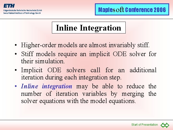
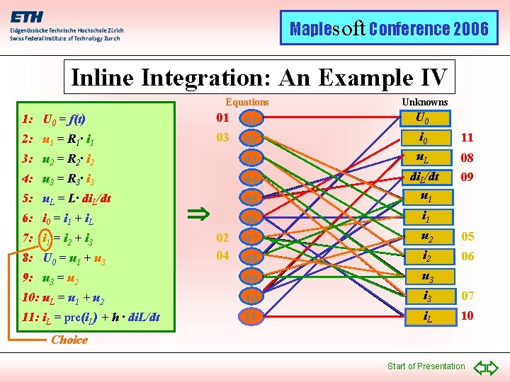
Maplesoft Conference 2006 Inline Integration • Higher-order models are almost invariably stiff. • Stiff models require an implicit ODE solver for their simulation. • Implicit ODE solvers call for an additional iteration during each integration step. • Inline integration may be able to reduce the number of iteration variables by merging the solver equations with the model equations. Start of Presentation

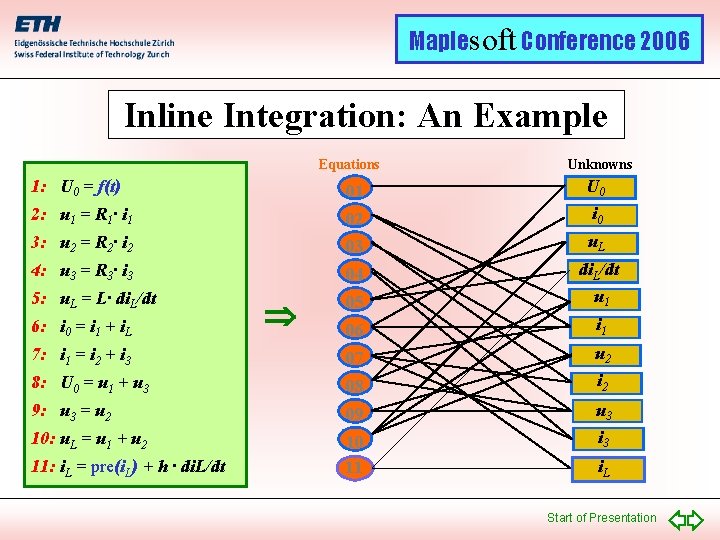
Maplesoft Conference 2006 Inline Integration: An Example Equations Unknowns 1: U 0 = f(t) 01 U 0 2: u 1 = R 1· i 1 02 i 0 3: u 2 = R 2· i 2 03 u. L 4: u 3 = R 3· i 3 04 5: u. L = L· di. L/dt 05 di. L/dt u 1 06 i 1 7: i 1 = i 2 + i 3 07 u 2 8: U 0 = u 1 + u 3 08 i 2 9: u 3 = u 2 09 u 3 10: u. L = u 1 + u 2 10 11 i 3 6: i 0 = i 1 + i. L 11: i. L = pre(i. L) + h · di. L/dt i. L Start of Presentation

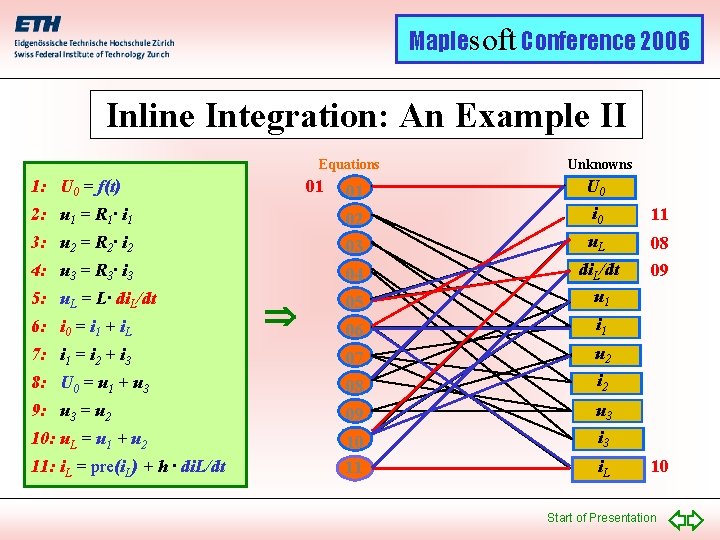
Maplesoft Conference 2006 Inline Integration: An Example II Equations 1: U 0 = f(t) Unknowns 01 U 0 2: u 1 = R 1· i 1 02 i 0 11 3: u 2 = R 2· i 2 03 u. L 08 4: u 3 = R 3· i 3 04 09 5: u. L = L· di. L/dt 05 di. L/dt u 1 06 i 1 7: i 1 = i 2 + i 3 07 u 2 8: U 0 = u 1 + u 3 08 i 2 9: u 3 = u 2 09 u 3 10: u. L = u 1 + u 2 10 11 i 3 6: i 0 = i 1 + i. L 11: i. L = pre(i. L) + h · di. L/dt 01 i. L 10 Start of Presentation

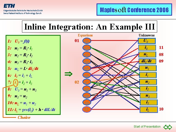
Maplesoft Conference 2006 Inline Integration: An Example III Equations Unknowns 01 U 0 2: u 1 = R 1· i 1 02 i 0 11 3: u 2 = R 2· i 2 03 u. L 08 4: u 3 = R 3· i 3 04 09 5: u. L = L· di. L/dt 05 di. L/dt u 1 06 i 1 07 u 2 8: U 0 = u 1 + u 3 08 i 2 9: u 3 = u 2 09 u 3 10: u. L = u 1 + u 2 10 11 i 3 01 1: U 0 = f(t) 6: i 0 = i 1 + i. L 7: i 1 = i 2 + i 3 11: i. L = pre(i. L) + h · di. L/dt 02 i. L 10 Choice Start of Presentation

Maplesoft Conference 2006 Inline Integration: An Example IV Equations Unknowns 1: U 0 = f(t) 01 01 U 0 2: u 1 = R 1· i 1 03 02 i 0 11 3: u 2 = R 2· i 2 03 u. L 08 4: u 3 = R 3· i 3 04 09 5: u. L = L· di. L/dt 05 di. L/dt u 1 06 i 1 07 u 2 05 08 i 2 06 9: u 3 = u 2 09 u 3 10: u. L = u 1 + u 2 10 11 i 3 07 i. L 10 6: i 0 = i 1 + i. L 7: i 1 = i 2 + i 3 8: U 0 = u 1 + u 3 11: i. L = pre(i. L) + h · di. L/dt 02 04 Choice Start of Presentation

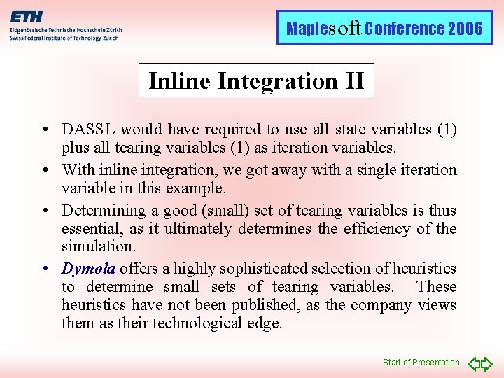
Maplesoft Conference 2006 Inline Integration II • DASSL would have required to use all state variables (1) plus all tearing variables (1) as iteration variables. • With inline integration, we got away with a single iteration variable in this example. • Determining a good (small) set of tearing variables is thus essential, as it ultimately determines the efficiency of the simulation. • Dymola offers a highly sophisticated selection of heuristics to determine small sets of tearing variables. These heuristics have not been published, as the company views them as their technological edge. Start of Presentation

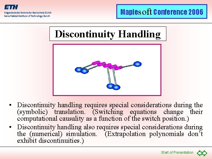
Maplesoft Conference 2006 Discontinuity Handling • Discontinuity handling requires special considerations during the (symbolic) translation. (Switching equations change their computational causality as a function of the switch position. ) • Discontinuity handling also requires special considerations during the (numerical) simulation. (Extrapolation polynomials don’t exhibit discontinuities. ) Start of Presentation

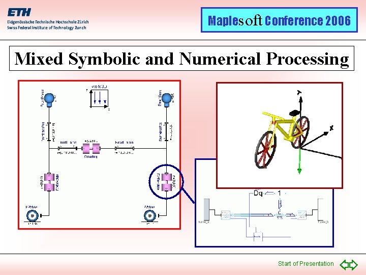
Maplesoft Conference 2006 Mixed Symbolic and Numerical Processing Start of Presentation