Internet Routing Architecture RIP OSPF Internet Routing Architecture

Internet Routing Architecture RIP & OSPF

Internet Routing Architecture 1. 2. 3. 4. Routing Intra-domain routing Inter-domain routing Convergence and Oscillation(papers)

Texts to read • 4. 2 -4. 3. 5 Peterson & Davie

Routing

Getting a datagram from source to dest. routing table in A Dest. Net. next router Nhops 223. 1. 1 223. 1. 2 223. 1. 3 IP datagram: misc source dest fields IP addr data • datagram remains unchanged, as it travels source to destination A B 223. 1. 1. 4 1 2 2 223. 1. 1. 1 223. 1. 1. 2 223. 1. 1. 4 223. 1. 1. 3 223. 1. 2. 9 223. 1. 3. 27 223. 1. 2. 2 223. 1. 3. 2 E

Getting a datagram from source to dest. misc data fields 223. 1. 1. 1 223. 1. 1. 3 Starting at A, given IP datagram addressed to B: • look up net. address of B • find B is on same net. as A • link layer will send datagram directly to B inside link-layer frame – B and A are directly connected Dest. Net. next router Nhops 223. 1. 1 223. 1. 2 223. 1. 3 A B 223. 1. 1. 4 1 2 2 223. 1. 1. 1 223. 1. 1. 2 223. 1. 1. 4 223. 1. 1. 3 223. 1. 2. 9 223. 1. 3. 27 223. 1. 2. 2 223. 1. 3. 2 E

Getting a datagram from source to dest. misc data fields 223. 1. 1. 1 223. 1. 2. 3 Dest. Net. next router Nhops 223. 1. 1 223. 1. 2 223. 1. 3 Starting at A, dest. E: • look up network address of E • E on different network – A, E not directly attached • routing table: next hop router to E is 223. 1. 1. 4 • link layer sends datagram to router 223. 1. 1. 4 inside linklayer frame • datagram arrives at 223. 1. 1. 4 A B 223. 1. 1. 4 1 2 2 223. 1. 1. 1 223. 1. 1. 2 223. 1. 1. 4 223. 1. 1. 3 223. 1. 2. 9 223. 1. 3. 27 223. 1. 2. 2 223. 1. 3. 2 E

Getting a datagram from source to dest. misc data fields 223. 1. 1. 1 223. 1. 2. 3 Arriving at 223. 1. 4, destined for 223. 1. 2. 2 • look up network address of E • E on same network as router’s interface 223. 1. 2. 9 – router, E directly attached • link layer sends datagram to 223. 1. 2. 2 inside link-layer frame via interface 223. 1. 2. 9 • datagram arrives at Dest. next network router Nhops interface 223. 1. 1 223. 1. 2 223. 1. 3 A B - 1 1 1 223. 1. 1. 4 223. 1. 2. 9 223. 1. 3. 27 223. 1. 1. 1 223. 1. 1. 2 223. 1. 1. 4 223. 1. 1. 3 223. 1. 2. 9 223. 1. 3. 27 223. 1. 2. 2 223. 1. 3. 2 E

Hierarchical routing

Hierarchical routing Inter-domain routing Intra-domain routing

Autonomous systems • What is an AS? – A set of routers under a single technical administration, using an interior gateway protocol (IGP) and common metrics to route packets within the AS and using an exterior gateway protocol (EGP) to route packets to other AS’s. – sometimes AS’s use multiple IGPs and metrics, but appear as single AS’s to other AS’s.

Example 1 2 IGP 1. 1 EGP 2. 2. 1 1. 2 EGP IGP 5 EGP 5. 2 EGP 3 3. 1 5. 1 2. 1 IGP 2. 2 IGP 3. 2 4. 1 IGP 4. 2 4

Routing Hierarchies • Flat routing doesn’t scale – Each node cannot be expected to have routes to every destination (or destination network) • Key observation – Need less information with increasing distance to destination • Two radically different approaches for routing – The area hierarchy – The landmark hierarchy

The Area Hierarchy 1 1. 1 2 2. 1 2. 2. 1 1. 2 3 3. 1 3. 2

Areas • Technique for hierarchically addressing nodes in a network • Divide network into areas – Areas can overlap – Areas can have nested sub-areas – Constraint: no path between two sub-areas of an area can exit that area • sub-areas must be completely contained within area

Addressing • Address areas hierarchically – sequentially number top-level areas – sub-areas of area are labeled relative to that area – nodes are numbered relative to the smallest containing area • nodes can have multiple addresses

Routing • Within area – each node has routes to every other node • Outside area – each node has routes for other top-level areas only – inter-area packets are routed to nearest border router • Can result in sub-optimal paths

Path Suboptimality 1 1. 1 2 2. 1 2. 2. 1 1. 2 3 3 hop red path vs 2 hop green path 2. 2 3. 1 3. 2

Intra-Domain Routing

Two main approaches • DV: Distance-vector protocols • LS: Link state protocols

Distance Vector Routing

Distance Vector Protocols • Employed in the early Arpanet • Distributed next hop computation – adaptive • Unit of information exchange – vector of distances to destinations • Distributed Bellman-Ford Algorithm

Distributed Bellman-Ford Start Conditions: (zero) distances to all directly attached networks (infinite) to other networks Send step: Each router advertises its current vector to all neighboring routers. Receive step: Upon receiving vectors from each of its neighbors, router computes its own distance to each neighbor. Then, for every network X, router finds that neighbor who is closer to X than to any other neighbor. Router updates its cost to X. After doing this for all X, router goes to send step.

Distance Vector (DV) Approach Consistency D(i, j) = c(i, k) + D(k, j) • The DV (Bellman-Ford) algorithm evaluates this recursion iteratively. – In the mth iteration, the consistency criterion holds, assuming that each node sees all nodes and links m-hops (or smaller) away from it (i. e. an m-hop view) 7 A B 1 2 8 1 E C 2 D Example network 7 A 1 B 7 A E B 1 C 8 1 E 2 D A’s 1 -hop view A’s 2 -hop view (After 1 st iteration) (After 2 nd Iteration)

Distance Vector (DV)… • Initial distance values (iteration 1): – D(i, i) = 0 ; – D(i, k) = c(i, k) if k is a neighbor (i. e. k is one-hop away); and – D(i, j) = INFINITY for all other non-neighbors j. • Note that the set of values D(i, *) is a distance vector at node i. • The algorithm also maintains a next-hop value (forwarding table) for every destination j, initialized as: – next-hop(i) = i; – next-hop(k) = k if k is a neighbor, and

Distance Vector (DV). . (Cont’d) • After every iteration each node i exchanges its distance vectors D(i, *) with its immediate neighbors. • For any neighbor k, if c(i, k) + D(k, j) < D(i, j), then: – D(i, j) = c(i, k) + D(k, j) – next-hop(j) = k • After each iteration, the consistency criterion is met – After m iterations, each node knows the shortest path possible to any other node which is m hops or less. – I. e. each node has an m-hop view of the network.

Example - initial distances 1 B C Info at node 7 8 A 1 E 2 2 D Distance to node A B C D E 0 7 ~ ~ 1 C 7 ~ 0 1 1 0 ~ 2 8 ~ D ~ ~ 2 0 2 E 1 8 ~ 2 0 A B

E receives D’s routes 1 B C Info at node 7 8 A 1 E 2 2 D Distance to node A B C D E 0 7 ~ ~ 1 C 7 ~ 0 1 1 0 ~ 2 8 ~ D ~ ~ 2 0 2 E 1 8 ~ 2 0 A B

E updates cost to C 1 B C Info at node 7 8 A 1 E 2 2 D Distance to node A B C D E 0 7 ~ ~ 1 C 7 ~ 0 1 1 0 ~ 2 8 ~ D ~ ~ 2 0 2 E 1 8 4 2 0 A B

A receives B’s routes 1 B C Info at node 7 8 A 1 E 2 2 D Distance to node A B C D E 0 7 ~ ~ 1 C 7 ~ 0 1 1 0 ~ 2 8 ~ D ~ ~ 2 0 2 E 1 8 4 2 0 A B

A updates cost to C 1 B C Info at node 7 8 A 1 E 2 2 D Distance to node A B C D E 0 7 8 ~ 1 C 7 ~ 0 1 1 0 ~ 2 8 ~ D ~ ~ 2 0 2 E 1 8 4 2 0 A B

A receives E’s routes 1 B C Info at node 7 8 A 1 E 2 2 D Distance to node A B C D E 0 7 8 ~ 1 C 7 ~ 0 1 1 0 ~ 2 8 ~ D ~ ~ 2 0 2 E 1 8 4 2 0 A B

A updates cost to C and D 1 B C Info at node 7 8 A 1 E 2 2 D Distance to node A B C D E 0 7 5 3 1 C 7 ~ 0 1 1 0 ~ 2 8 ~ D ~ ~ 2 0 2 E 1 8 4 2 0 A B

Final distances 1 B C Info at node 7 8 A 1 E 2 2 D Distance to node A B C D E 0 6 5 3 1 C 6 5 0 1 1 0 3 2 5 4 D 3 3 2 0 2 E 1 5 4 2 0 A B

Final distances after link failure 1 B C Info at node 7 8 A 1 E 2 2 D Distance to node A B C D E A B 0 7 8 10 1 7 0 1 3 8 C 8 1 0 2 9 D 10 3 2 0 11 E 1 9 11 0 8

View from a node 1 B E’s routing table Next hop C 7 8 A 1 E 2 2 D dest A B D A B 1 14 5 C 7 6 8 9 5 4 D 4 11 2

The bouncing effect dest cost B C 1 2 dest cost 1 A B 1 25 C dest cost A B 2 1 A C 1 1

C sends routes to B dest Cost: nhop dest cost B C 1 2 A B 1 25 C dest Cost: nhop A B 2: B 1 A C ~ 1

B updates distance to A dest Cost: nhop dest cost B C 1 2 A B 1 25 C dest Cost: nhop A B 2: B 1 A C 3: C 1

B sends routes to C dest Cost: nhop dest cost B C 1 2 A B 1 25 C dest cost A B 4: B 1 A C 3: C 1

C sends routes to B dest Cost: nhop dest cost B C 1 2 A B 1 25 C dest Cost: nhop A B 4: B 1 A C 5: C 1

Distance Vector: link cost Link cost changes: changes 1 q node detects local link cost 4 change X q updates distance table q if cost change in least cost path, notify neighbors “good Time 0 Iter. 1 Iter. 2 news travels DV(Y) [ 4 0 1] [ 1 0 1] fast” DV(Z) [ 5 1 0] [ 1 0 1] [ 2 1 0] Y 50 1 Z algorithm terminates

Distance Vector: link cost Link cost changes: changes q good news travels fast q bad news travels slow “count to infinity” problem! Time 0 Iter 1 Iter 2 60 X 4 Iter 3 Y 50 1 Z Iter 4 DV(Y) [ 4 0 1] [ 6 0 1] [ 8 0 1] DV(Z) [ 5 1 0] [ 7 1 0] [ 9 1 0] algo goes on!

Distance Vector: poisoned reverse q If Z routes through Y to get to X : 60 4 q. Z tells Y its (Z’s) distance to X is infinite (so Y won’t route to X via Z) X q. At Time 0, DV(Z) as seen by Y is [INF 0], not [5 1 0] ! Time 0 Y 50 Iter 1 Iter 2 Iter 3 DV(Y) [ 4 0 1] [ 60 0 1] [ 51 0 1] DV(Z) [ 5 1 0] [ 50 1 0] [ 7 1 0] [ 5 1 0] 1 Z algorithm terminates

How are these loops caused? • Observation 1: – B’s metric increases • Observation 2: – C picks B as next hop to A – But, the implicit path from C to A includes itself!

Solution 1: Holddowns • If metric increases, delay propagating information – in our example, B delays advertising route – C eventually thinks B’s route is gone, picks its own route – B then selects C as next hop • Adversely affects convergence

Other “solutions” • Split horizon – B does not advertise route to C • Poisoned reverse – B advertises route to C with infinite distance • Works for two node loops – does not work for loops with more nodes

Example A B 1 5 1 C D 1

Distance Vector (DV) Example • A’s distance vector D(A, *): – – 7 A After Iteration 1 is: After Iteration 2 is: After Iteration 3 is: After Iteration 4 is: B 1 1 E C 2 8 2 [0, 7, INFINITY, 1] [0, 7, 8, 3, 1] [0, 7, 5, 3, 1] [0, 6, 5, 3, 1] D Example network 7 A 1 B 7 A E B 1 C 8 1 E 2 D A’s 1 -hop view A’s 2 -hop view (After 1 st iteration) (After 2 nd Iteration)

Avoiding the Bouncing Effect • Select loop-free paths • One way of doing this: – each route advertisement carries entire path – if a router sees itself in path, it rejects the route • BGP does it this way – Space proportional to diameter Cheng, Riley et al

Computing Implicit Paths • To reduce the space requirements – propagate for each destination not only the cost but also its predecessor – can recursively compute the path – space requirements independent of diameter v x y z w u

Loop Freedom at Every Instant • Does bouncing effect avoid loops? – No! Transient loops are still possible – Why? Because implicit path information may be stale • Only way to fix this – ensure that you have up-to-date information by explicitly querying

Distance Vector in Practice • RIP and RIP 2 – uses split-horizon/poison reverse • BGP/IDRP – propagates entire path – path also used for effecting policies

RIP ( Routing Information Protocol) • Distance vector algorithm • Included in BSD-UNIX Distribution in 1982 • Distance metric: # of hops (max = 15 hops) – Can you guess why? • Distance vectors: exchanged every 30 sec via Response Message (also called advertisement) • Each advertisement: route to up to 25 destination nets

RIP (Routing Information Protocol) z w A x D B y C Destination Network w y z x …. Next Router Num. of hops to dest. …. . . A B B -- Routing table in D 2 2 7 1

RIP: Link Failure and Recovery If no advertisement heard after 180 sec --> neighbor/link declared dead – routes via neighbor invalidated – new advertisements sent to neighbors – neighbors in turn send out new advertisements (if tables changed) – link failure info quickly propagates to entire net – poison reverse used to prevent ping-pong loops (infinite distance = 16 hops)

RIP Table processing • RIP routing tables managed by application-level process called route-d (daemon) • advertisements sent in UDP packets, periodically repeated

RIP Table example (continued) Router: giroflee. eurocom. fr Destination ----------127. 0. 0. 1 192. 168. 2. 193. 55. 114. 192. 168. 3. 224. 0. 0. 0 default • • • Gateway Flags Ref Use Interface ---------- --------127. 0. 0. 1 UH 0 26492 lo 0 192. 168. 2. 5 U 2 13 fa 0 193. 55. 114. 6 U 3 58503 le 0 192. 168. 3. 5 U 2 25 qaa 0 193. 55. 114. 6 U 3 0 le 0 193. 55. 114. 129 UG 0 143454 Three attached class C networks (LANs) Router only knows routes to attached LANs Default router used to “go up” Route multicast address: 224. 0. 0. 0 Loopback interface (for debugging)

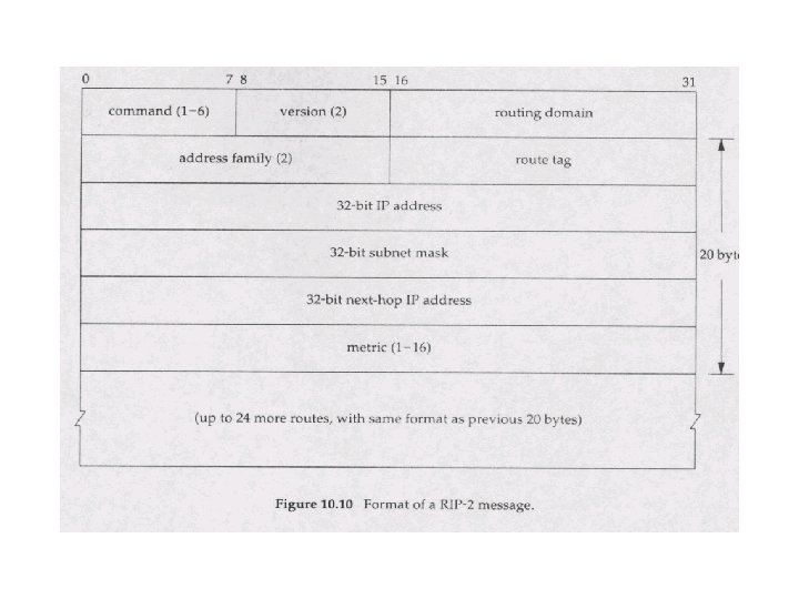
RIP v 2 • Use “must be zero” fields • routing daemon: identifier, process ID(Unix), allows for multiple RIPs on a single router, each operating within one routing domain • route tag: carries AS number for EGP and BGP • subnet mask, next hop, authentication, multicast

IGRP (Interior Gateway Routing Protocol) • CISCO proprietary; successor of RIP (mid 80 s) • Distance Vector, like RIP • several cost metrics (delay, bandwidth, reliability, load etc) • uses TCP to exchange routing updates • Loop-free routing via Distributed Updating Alg. (DUAL) based on diffused computation

Link-state Routing

Basic steps • Each node assumed to know state of links to its neighbors • Step 1: Each node broadcasts its state to all other nodes • Step 2: Each node locally computes shortest paths to all other nodes from global state

Building blocks • Reliable broadcast mechanism – flooding – sequence number issues • Shortest path tree (SPT) algorithm – Dijkstra’s SPT algorithm

Link state packets (LSPs) • Periodically, each node creates a Link state packet containing: – Node ID – List of neighbors and link cost – Sequence number – Time to live (TTL) • Node outputs LSP on all its links

Reliable flooding • When node i receives LSP from node j: – If LSP is the most recent LSP from j that i has seen so far, i saves it in database and forwards a copy on all links except link LSP was received on. – Otherwise, discard LSP.

Sequence number space issues • Problem: sequence number may wrap around • Solution: treat space as circular, continue after wrap around: – A is less than B if • A<B and B-A < N/2, or • A>B and A-B > N/2 B A 0 N Wrap around

Problem: Router Failure • A failed router and comes up but does not remember the last sequence number it used before it crashed • New LSPs may be ignored if they have lower sequence number

One solution: LSP Aging • Nodes periodically decrement age (TTL) of stored LSPs • LSPs expire when TTL reaches 0 – LSP is re-flooded once TTL = 0 • Rebooted router waits until all LSPs have expired • Trade-off between frequency of LSPs and router wait after reboot

OSPF Sequencing and Aging • • 32 -bit sequence number field, does not wrap LSP’s compared on basis of sequence number LSP’s purged after about an hour Synchronized expiration of LSPs – expired LSP reflooded with age zero • On startup, router need not wait – can start with lowest sequence number – will be informed if its own LSP is in network

SPT algorithm (Dijkstra) • SPT = {a} • for all nodes v – if v adjacent to a then D(v) = cost (a, v) – else D(v) = infinity • Loop – find w not in SPT, where D(w) is min – add w in SPT – for all v adjacent to w and not in SPT • D(v) = min (D(v), D(w) + C(w, v)) • until all nodes are in SPT

Example 5 B 2 A 3 2 1 D B 1 C 3 1 C E D 5 F 2 E F

Example 5 B 2 A 3 2 1 D B 1 C 3 1 C E D 5 F 2 E F

Example 5 B 2 A 3 2 1 D B 1 C 3 1 C E D 5 F 2 E F

Example 5 B 2 A 3 2 1 D B 1 C 3 1 C E D 5 F 2 E F

Example 5 B 2 A 3 2 1 D B 1 C 3 1 C E D 5 F 2 E F

Example 5 B 2 A 3 2 1 D B 1 C 3 1 C E D 5 F 2 E F

Link State Algorithm Flooding: 1) Periodically distribute link-state advertisement (LSA) to neighbors - LSA contains delays to each neighbor 2) Install received LSA in LS database 3) Re-distribute LSA to all neighbors Path Computation 1) Use Dijkstra’s shortest path algorithm to compute distances to all destinations 2) Install <destination, nexthop> pair in forwarding table

Link State Characteristics • With consistent LSDBs, all nodes compute consistent loop-free paths • Limited by Dijkstra computation overhead, space requirements B • Can still have transient loops 1 Packet from C->A may loop around BDC A 1 3 5 C 2 D

OSPF (Open Shortest Path First) • “open”: publicly available • Uses Link State algorithm – LS packet dissemination – Topology map at each node – Route computation using Dijkstra’s algorithm • OSPF advertisement carries one entry per neighbor router • Advertisements disseminated to entire AS (via flooding)

OSPF “advanced” features (not in RIP) • Security: all OSPF messages authenticated (to prevent malicious intrusion); TCP connections used • Multiple same-cost paths allowed (only one path in RIP) • For each link, multiple cost metrics for different TOS (eg, satellite link cost set “low” for best effort; high for real time) • Integrated uni- and multicast support: – Multicast OSPF (MOSPF) uses same topology data base as OSPF • Hierarchical OSPF in large domains.

Hierarchical OSPF

Hierarchical OSPF • Two-level hierarchy: local area, backbone. – Link-state advertisements only in area – each nodes has detailed area topology; only know direction (shortest path) to nets in other areas. • Area border routers: “summarize” distances to nets in own area, advertise to other Area Border routers. • Backbone routers: run OSPF routing limited to backbone. • Boundary routers: connect to other ASs.

LS v. s. DV In DV send everything you know to your neighbors. In LS send info about your neighbors to everyone. • Msg size: small with LS, potentially large with DV • Msg exchange: LS: O(n. E), DV: only to neighbors

LS v. s. DV • Convergence speed: – LS: fast – DV: fast with triggered updates • Space requirements: – LS maintains entire topology – DV maintains only neighbor state

LS v. s. DV Robustness: • LS can broadcast incorrect/corrupted LSP – localized problem • DV can advertise incorrect paths to all destinations – incorrect calculation can spread to entire network

LS v. s. DV • In LS notes must compute consistent routes independently - must protect against LSDB corruption • In DV routes are computed relative to other nodes Bottom line: no clear winner, but we see more frequent use of LS in the Internet

The ARPANET Experience

Importance of cost metric • Choice of link cost defines traffic load – low cost = high probability link belongs to SPT and will attract traffic • Main problem: convergence – avoid oscillations – good network utilization

Metric choices • Static metrics (e. g. , hop count) – good only if links are homogeneous – not the case in the Internet • Static metrics do not take into account: – link delay – link capacity – link load (hard to measure)

Original ARPANET metric • Cost proportional to queue size – instantaneous queue length as delay estimator • Problems: – did not take into account link speed – poor indicator of expected delay due to rapid fluctuations – delay may be longer even if queue size is small due to contention for other resources

New metric • Delay = (depart time - arrival time) + transmission time + link propagation delay – (depart time - arrival time) captures queuing – transmission time captures link capacity – link propagation delay captures the physical length of the link • Measurements averaged over 10 seconds – Update sent if difference > threshold, or every 50 seconds

Performance of new metric • Works well for light to moderate load – static values dominate • Oscillates under heavy load – queuing dominates • Reason: there is no correlation between original and new values of delay after rerouting!

Specific problems • Range is too wide – 9. 6 Kbps highly loaded link can appear 127 times costlier than 56 Kbps lightly loaded link – can make a 127 -hop path look better than 1 -hop • No limit in reported delay variation • All nodes calculate routes simultaneously – triggered by link update

Example A Net X Net Y B

. . example After everyone re-calculates routes: A Net X Net Y B . . Oscillations!

Consequences • Low network utilization (50% in example) • Congestion can spread elsewhere • Routes could oscillate between short and long paths • Large swings lead to frequent route updates – more messages – frequent SPT re-calculation

Revised link metric • Better metric: packet delay = f(queueing, transmission, propagation). • When lightly loaded, transmission and propagation are good predictors • When heavily loaded queueing delay is dominant and so transmission and propagation are bad predictors

Normalized metric (Zinky et al) • If a loaded link looks very bad then everyone will move off of it • Want some to stay on to load balance and avoid oscillations • It is still an OK path for some • Hop normalized metric diverts routes that have an alternate that is not too much longer • Also limited relative values and range of values advertised…gradual change

Revised Metric (cont. ) • Average utilization measures limit range of change…. 5*sample +. 5*last average • Normalize according to link type (eg satellite should look good as queueing on other links increase) • Max change allowed is link type specific – change per update cannot be more than 1/2 of that hops delay value (e. g. max is 90 and min is 30 so worst case is only 2 hops worse than best)

New metric (routing units) Routing metric v. s. link utilization 225 140 90 75 60 30 0 9. 6 satellite 9. 6 terrestrial 56 satellite 56 terrestrial 25% 50% 75% 100% Utilization

Observations • Cost of highly loaded link never more than 3*cost when idle • Most expensive link is 7 * least expensive link • High-speed satellite link is more attractive than low-speed terrestrial link

. . observations • Cost = f(link utilization) only at moderate to high loads • Allows routes to be gradually shed from link – also takes into account link characteristics

Network response maps Load 1. 0 200% 0. 75 100% 0. 5 50% 0. 25 0 25% 0. 5 1. 0 1. 5 2. 0 2. 5 3. 0 3. 5 4. 0 Metric Load of “average” link as a function of that link’s cost Created empirically

Routing dynamics Utilization Metric map Bounded oscillation 1. 0 0. 75 0. 5 Network response 0. 25 0 0. 5 1. 0 1. 5 2. 0 2. 5 3. 0 3. 5 4. 0 Link reported cost

Routing dynamics Utilization Metric map 1. 0 0. 75 Easing in a new link 0. 5 Network response 0. 25 0 0. 5 1. 0 1. 5 2. 0 2. 5 3. 0 3. 5 4. 0 Reported cost

Synchronization of Routing Messages

Routing Update Synchronization • Another interesting robustness issue to consider. . . • Even apparently independent processes can eventually synchronize – e. g. periodic routing protocol messages from different routers • Features: – abrupt transition from unsychronized to synchronized system states – can be broken up by introducing randomization

Examples of Occurrence • TCP congestion windows – cyclical behavior shared by flows through gateway • External events – periodic downloads • Synchronized client restart – e. g. after a catastrophic failure • Periodic routing messages – manifests itself as periodic packet losses on end-to-end pings

How can routing messages synchronize? T A Message from B T Weak Coupling when A’s behavior is triggered off of B’s message arrival! A Weak coupling can result in eventual synchronization No Coupling when A sends at a time that is independent of B’s message arrival

Periodic message model • Router prepares and sends update, resets timer Tc seconds after start time; received by other routers Td seconds from start • If router receives incoming routing update while preparing its own, router processes incoming update. Tc 2 seconds to process • After generating update set timer drawn uniformly from [Tp-Tr, Tp+Tr] seconds, Tp is avg period, Tr random component. When timer expires repeat. If update occurs reflecting topology event, repeat also. Why is this a problem? ? ?

Routing source of synchronization • Router resets timer after processing its own and incoming updates • Creates weak coupling among routers! • There are solutions: – set timer based on clock event that is not a function of processing other routers’ updates, or – add randomization, or reset timer before processing update

Analyzing Synchronization • Three step approach – design a model that captures the essential behavior – study the parameter space under a simulation – simplify the model to make it analytically tractable

The Periodic Message Model A’s routing update A Tc Others’ routing updates Tc 2 Td [Tp-Tr, Tp+Tr]

What Happens?

Why Does it Happen?

Important Results • With increasing Tr (randomization) – takes longer to synchronize – may need Tr to be ten times Tc • A robust choice of timer Tr = Tp/2 • With increasing randomization, abrupt transition – from predominantly synchronized to predominantly unsynchronized

Musings • Other self-synchronizing phenomena – pendulum clocks – automobile traffic patterns • Emergent large-scale structure likely to result from more complex system interactions • Will be interesting to watch for this in the context of “micronets”