II INTERFIRM RELATIONSHIPS AND THE INTENSIVE MARGIN OF

II. INTERFIRM RELATIONSHIPS AND THE INTENSIVE MARGIN OF BILATERAL TRADE James E. Rauch The Nottingham Lectures in International Economics

Connection to previous lecture • Interfirm matching, and the impact of information on trade through that matching • Nothing comparable to m, a measure of international networks that make international matching as perfect as domestic matching. Instead, the impact of interpersonal relationships is only implicit through the impact of distance or colonial ties on the matching process (Head et al. 2009) • Preliminary work, comments welcome

The Melitz heterogeneous firm model and bilateral trade • The Melitz (2003) model of international trade with heterogeneous firms has now become part of our standard toolkit • The model was designed to show trade liberalization could raise average firm productivity, but has run into some problems as its application has been extended to the extensive margin (number of firms/varieties) and intensive margin (value of trade per firm/variety) of bilateral trade

Bilateral fixed or variable costs • Hanson and Xiang (2009) have brought out these problems especially clearly in their study of U. S. bilateral exports of motion pictures. • They begin by making the point, “Standard gravity variables – distance, language, colonial history – are likely correlated with variable and fixed barriers” to bilateral trade • It follows that to predict the impact of bilateral distance, say, on the bilateral extensive and intensive margin, one must consider its effects through both bilateral fixed and variable costs

Impacts of bilateral fixed costs • Bilateral fixed costs decrease bilateral trade at the extensive margin, but increase bilateral trade at the intensive margin • The higher are bilateral fixed costs, the fewer exporting firms find it worthwhile to export from country i to country j • It follows that the productivity (size) of the cutoff exporter increases with bilateral fixed costs, so that the average value of bilateral exports per firm increases

Impacts of bilateral variable costs • Bilateral variable costs decrease bilateral trade at the extensive margin for the same reason as bilateral fixed costs • Bilateral variable costs have offsetting effects on the intensive margin. Each exporting firm exports a lower value, but the cutoff exporting firm is larger • With the standard assumption that firm size is Pareto distributed, the two effects of variable costs on the average value of bilateral exports per firm exactly cancel

Predicted impacts of distance • Consider a variable such as distance that is positively correlated with variable costs of bilateral trade and (weakly) positively correlated with fixed costs of bilateral trade • This variable unambiguously reduces bilateral trade at the extensive margin. With a Pareto distribution of firm size, it (weakly) increases bilateral trade at the intensive margin • As we shall see, this prediction is strongly counterfactual

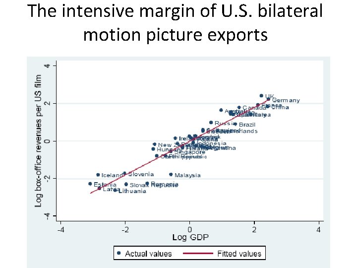
Impacts of importer market size • Less emphasized by Hanson and Xiang are the predictions of the Melitz model for the effects of importer market size (GNP) on the extensive and intensive margins of bilateral trade • Larger importer market size works analogously to lower variable bilateral trade costs, hence is predicted to increase bilateral trade at the extensive margin while leaving the intensive margin unchanged (if the firm size distribution is Pareto) • Zero impact of importer GNP on the average value of exports per firm that exports to the importer is the most strongly counterfactual prediction of all

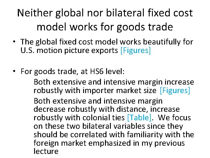
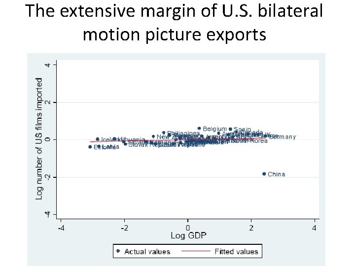
Global versus bilateral fixed costs • For motion picture exports, Hanson and Xiang propose a model of global instead of bilateral fixed costs. Firms pay a fixed cost to enter the world market, but no additional fixed cost per country • The result is that only the better firms export (only the better films are exported), as in the standard heterogeneous firm model, but the extensive margin (number of films imported) does not vary across importers • The intensive margin, on the other hand, varies across importers in the intuitive way with respect to market size, distance, etc.

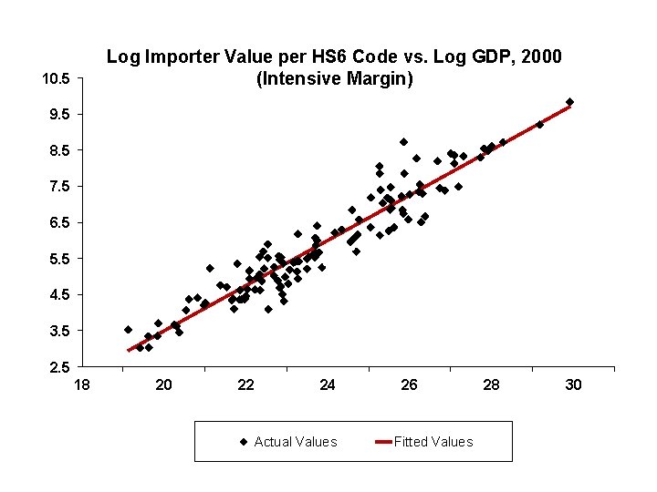
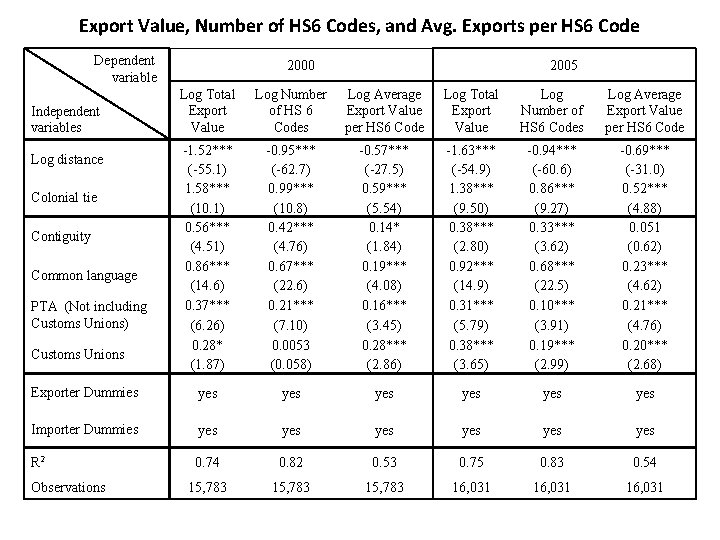
Neither global nor bilateral fixed cost model works for goods trade • The global fixed cost model works beautifully for U. S. motion picture exports [Figures] • For goods trade, at HS 6 level: Both extensive and intensive margin increase robustly with importer market size [Figures] Both extensive and intensive margin decrease robustly with distance, increase robustly with colonial ties [Table]. We focus on these two bilateral variables since they should be correlated with familiarity with the foreign market emphasized in my previous lecture

The extensive margin of U. S. bilateral motion picture exports

The intensive margin of U. S. bilateral motion picture exports

Log Importer HS 6 Count vs. Log GDP, 2000 (Extensive Margin) 12. 5 12 11. 5 11 10. 5 10 9. 5 9 8. 5 8 18 20 22 24 Actual Values 26 28 Fitted Values 30

Log Importer Value per HS 6 Code vs. Log GDP, 2000 (Intensive Margin) 10. 5 9. 5 8. 5 7. 5 6. 5 5. 5 4. 5 3. 5 2. 5 18 20 22 24 Actual Values 26 Fitted Values 28 30

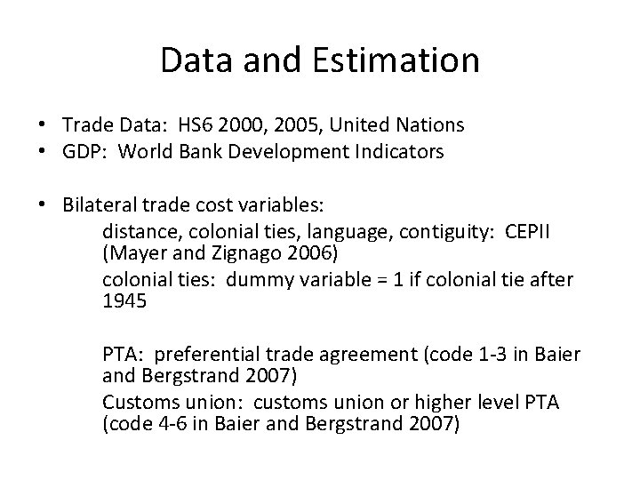
Data and Estimation • Trade Data: HS 6 2000, 2005, United Nations • GDP: World Bank Development Indicators • Bilateral trade cost variables: distance, colonial ties, language, contiguity: CEPII (Mayer and Zignago 2006) colonial ties: dummy variable = 1 if colonial tie after 1945 PTA: preferential trade agreement (code 1 -3 in Baier and Bergstrand 2007) Customs union: customs union or higher level PTA (code 4 -6 in Baier and Bergstrand 2007)

Export Value, Number of HS 6 Codes, and Avg. Exports per HS 6 Code Dependent variable 2000 2005 Log Total Export Value Log Number of HS 6 Codes Log Average Export Value per HS 6 Code -1. 52*** (-55. 1) 1. 58*** (10. 1) 0. 56*** (4. 51) 0. 86*** (14. 6) 0. 37*** (6. 26) 0. 28* (1. 87) -0. 95*** (-62. 7) 0. 99*** (10. 8) 0. 42*** (4. 76) 0. 67*** (22. 6) 0. 21*** (7. 10) 0. 0053 (0. 058) -0. 57*** (-27. 5) 0. 59*** (5. 54) 0. 14* (1. 84) 0. 19*** (4. 08) 0. 16*** (3. 45) 0. 28*** (2. 86) -1. 63*** (-54. 9) 1. 38*** (9. 50) 0. 38*** (2. 80) 0. 92*** (14. 9) 0. 31*** (5. 79) 0. 38*** (3. 65) -0. 94*** (-60. 6) 0. 86*** (9. 27) 0. 33*** (3. 62) 0. 68*** (22. 5) 0. 10*** (3. 91) 0. 19*** (2. 99) -0. 69*** (-31. 0) 0. 52*** (4. 88) 0. 051 (0. 62) 0. 23*** (4. 62) 0. 21*** (4. 76) 0. 20*** (2. 68) Exporter Dummies yes yes yes Importer Dummies yes yes yes R 2 0. 74 0. 82 0. 53 0. 75 0. 83 0. 54 15, 783 16, 031 Independent variables Log distance Colonial tie Contiguity Common language PTA (Not including Customs Unions) Customs Unions Observations

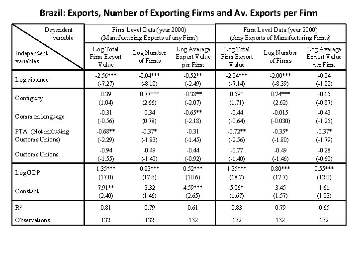
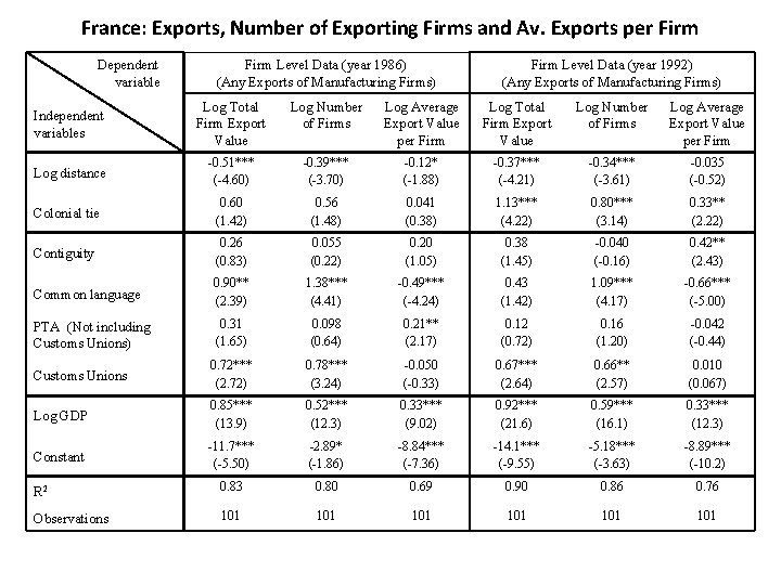
Firm level results support HS 6 level results • The intensive margin results at the HS 6 level may conflate the extensive with the intensive margin, because there are many firms/varieties per HS 6 bilateral import • We therefore checked the intensive (and extensive) margin results against whatever firm level data we were able to obtain. • Marc Muendler and Sam Kortum respectively supplied Brazilian and French firm level export data • Following my previous lecture, the firm level will best match theory we develop [Tables]

Brazil: Exports, Number of Exporting Firms and Av. Exports per Firm Dependent variable Firm Level Data (year 2000) (Manufacturing Exports of any Firm) Firm Level Data (year 2000) (Any Exports of Manufacturing Firms) Independent variables Log Total Firm Export Value Log Number of Firms Log Average Export Value per Firm Log distance -2. 56*** (-7. 27) -2. 04*** (-8. 18) -0. 52** (-2. 49) -2. 24*** (-7. 14) -2. 00*** (-8. 39) -0. 24 (-1. 22) Contiguity 0. 39 (1. 04) 0. 77*** (2. 66) -0. 38** (-2. 07) 0. 59* (1. 71) 0. 74*** (2. 62) -0. 15 (-0. 87) Common language -0. 31 (-0. 56) 0. 34 (0. 78) -0. 65** (-2. 18) -0. 44 (-0. 64) -0. 015 (-0. 030) -0. 43 (-1. 25) PTA (Not including Customs Unions) -0. 68** (-2. 29) -0. 37* (-1. 83) -0. 31 (-1. 45) -0. 72** (-2. 56) -0. 35* (-1. 80) -0. 37* (-1. 79) Customs Unions -0. 94 (-1. 55) -0. 49 (-1. 40) -0. 44 (-0. 92) -0. 77 (-1. 40) -0. 49 (-1. 46) -0. 28 (-0. 60) Log GDP 1. 35*** (17. 0) 0. 83*** (17. 6) 0. 52*** (10. 6) 1. 35*** (18. 7) 0. 80*** (17. 7) 0. 55*** (12. 0) Constant 7. 91** (2. 40) 3. 32 (1. 46) 4. 59*** (2. 65) 5. 06* (1. 67) 3. 45 (1. 57) 1. 61 (1. 03) R 2 0. 81 0. 79 0. 61 0. 83 0. 79 0. 65 Observations 132 132 132

France: Exports, Number of Exporting Firms and Av. Exports per Firm Dependent variable Firm Level Data (year 1986) (Any Exports of Manufacturing Firms) Firm Level Data (year 1992) (Any Exports of Manufacturing Firms) Independent variables Log Total Firm Export Value Log Number of Firms Log Average Export Value per Firm Log distance -0. 51*** (-4. 60) -0. 39*** (-3. 70) -0. 12* (-1. 88) -0. 37*** (-4. 21) -0. 34*** (-3. 61) -0. 035 (-0. 52) Colonial tie 0. 60 (1. 42) 0. 56 (1. 48) 0. 041 (0. 38) 1. 13*** (4. 22) 0. 80*** (3. 14) 0. 33** (2. 22) Contiguity 0. 26 (0. 83) 0. 055 (0. 22) 0. 20 (1. 05) 0. 38 (1. 45) -0. 040 (-0. 16) 0. 42** (2. 43) Common language 0. 90** (2. 39) 1. 38*** (4. 41) -0. 49*** (-4. 24) 0. 43 (1. 42) 1. 09*** (4. 17) -0. 66*** (-5. 00) PTA (Not including Customs Unions) 0. 31 (1. 65) 0. 098 (0. 64) 0. 21** (2. 17) 0. 12 (0. 72) 0. 16 (1. 20) -0. 042 (-0. 44) Customs Unions 0. 72*** (2. 72) 0. 78*** (3. 24) -0. 050 (-0. 33) 0. 67*** (2. 64) 0. 66** (2. 57) 0. 010 (0. 067) Log GDP 0. 85*** (13. 9) 0. 52*** (12. 3) 0. 33*** (9. 02) 0. 92*** (21. 6) 0. 59*** (16. 1) 0. 33*** (12. 3) Constant -11. 7*** (-5. 50) -2. 89* (-1. 86) -8. 84*** (-7. 36) -14. 1*** (-9. 55) -5. 18*** (-3. 63) -8. 89*** (-10. 2) R 2 0. 83 0. 80 0. 69 0. 90 0. 86 0. 76 Observations 101 101 101

Exporters matching with importing firms is a natural fix • These problems with the Melitz model can probably be fixed by tweaking the model in various ways • However, just one change will fix all the problems while moving the model unambiguously in the direction of realism: having exporters match with importing firms rather than sell directly to consumers • Importing firms may be manufacturers purchasing intermediates, retailers buying final goods, or distributors marketing to manufacturers or retailers

Match quality • We will assume that the exporting and importing firms jointly draw a match quality. This can be affected by any bilateral variable that influences search cost or familiarity. For example, if greater distance increases search costs and/or reduces familiarity, it will worsen the distribution of match quality, thereby decreasing trade at both the intensive and extensive margins. • We will adhere to the assumption of a Pareto distribution of (match) productivity and model greater familiarity as a first-order stochastic dominant shift in that distribution. The same cutoff level of productivity (match quality) then corresponds to more confirmed matches and a higher average match quality

Opportunity cost • Using data that matches all Chilean exporters with their Colombian importers for 2004 -2006, Blum et al (2009) find that in virtually all matches at least one of the parties is large • This is usually the importer: more than half of the Chilean exporters sell to only one Colombian importer, and these importers purchase larger amounts and more HS codes than other importers • We assume that any importer optimizes its “scope, ” the number of varieties it markets. If it takes on a new imported variety, it must give up or at least reduce sales of another variety, either domestic or imported. • This tradeoff (opportunity cost) will be proportional to domestic market size. In combination with bilateral fixed costs unrelated to market size (e. g. , paperwork to comply with regulations), importing firms then lead to trade increasing with market size at the intensive as well as extensive margin • A similar logic should apply if the exporter is the large party, large enough to have power in the market of the importing country. However, we have not proved this

Model of marketing, with production in the background • Each export variety from country i is handled by a sales representative, who is supplied at constant cost ci by a manufacturer, where ci can include a markup. Hereafter we refer to the sales representative as the exporter • The representative importer-wholesaler or retailer in country j faces the standard CES demand for any variety it markets, domestic or foreign. Hereafter we refer to this firm as the importer • Exporters from i match randomly with importers from j. If the match is unsuccessful, each gets zero – that variety is not traded between i and j • We denote the quality of a match between an exporter and an importer by z, which acts like productivity in the Melitz model: it divides the marginal cost of supplying the exported variety to j

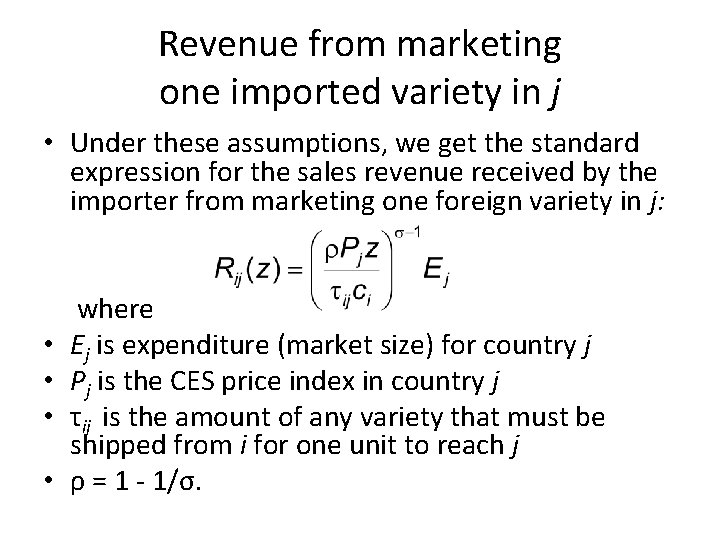
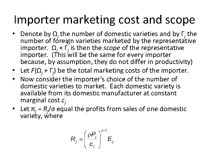
Revenue from marketing one imported variety in j • Under these assumptions, we get the standard expression for the sales revenue received by the importer from marketing one foreign variety in j: • • where Ej is expenditure (market size) for country j Pj is the CES price index in country j τij is the amount of any variety that must be shipped from i for one unit to reach j ρ = 1 - 1/σ.

Benefits and costs of confirming a match • We have the standard CES relationship between profit and revenue: πij(z) = Rij(z)/σ • In order for the match to be successful, this must exceed the costs of establishing the exporter-importer relationship • This includes a bilateral fixed cost fij ≥ 0, which might include the cost of regulatory compliance, say. This might be unaffected by distance (all paperwork is done electronically) or positively affected by distance (meetings are required) • If the importer is a multiproduct firm, as we shall assume, there is also an opportunity cost for it to market an additional variety, as discussed earlier. We now model this opportunity cost

Domestic and foreign varieties • We assume, crucially, that the importer can vary the number of domestic varieties it markets so as to maximize profits, but encounters opportunities to market foreign varieties only through random matching. This assumption mirrors the assumption of perfect domestic matching and random foreign matching made in yesterday’s lecture • Following Arkolakis and Muendler (2009), the importer incurs marketing costs for its varieties that increase in the number of varieties but do not depend on the quantity sold per variety. We can think of these as the costs of developing promotional campaigns • In general, the importer will also have to consider the possibility that each additional variety it markets will cannibalize demand for its other varieties. For simplicity, however, we assume that the importer is too small relative to the entire domestic market to affect the domestic price level Pj

Importer marketing cost and scope • Denote by Ωj the number of domestic varieties and by Гj the number of foreign varieties marketed by the representative importer. Ωj + Гj is then the scope of the representative importer. (This will be the same for every importer because, by assumption, they do not differ in productivity) • Let F(Ωj + Гj) be the total marketing costs of the importer. • Now consider the importer’s choice of the number of domestic varieties to market. Each domestic variety is available from its domestic manufacturer at constant marginal cost cj • Let πj = Rj/σ equal the profits from sales of one domestic variety, where

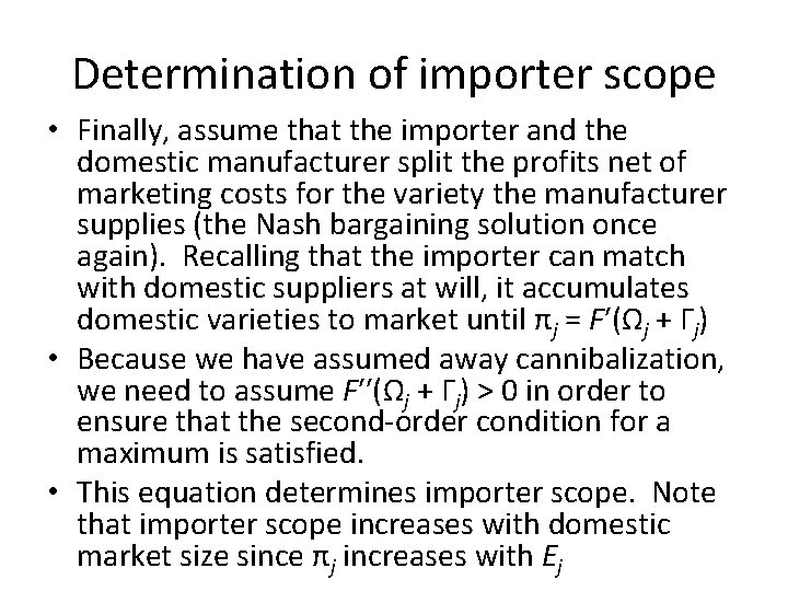
Determination of importer scope • Finally, assume that the importer and the domestic manufacturer split the profits net of marketing costs for the variety the manufacturer supplies (the Nash bargaining solution once again). Recalling that the importer can match with domestic suppliers at will, it accumulates domestic varieties to market until πj = F′(Ωj + Гj) • Because we have assumed away cannibalization, we need to assume F′′(Ωj + Гj) > 0 in order to ensure that the second-order condition for a maximum is satisfied. • This equation determines importer scope. Note that importer scope increases with domestic market size since πj increases with Ej

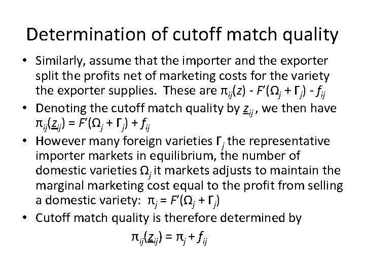
Determination of cutoff match quality • Similarly, assume that the importer and the exporter split the profits net of marketing costs for the variety the exporter supplies. These are πij(z) - F′(Ωj + Гj) - fij • Denoting the cutoff match quality by zij , we then have πij(zij) = F′(Ωj + Гj) + fij • However many foreign varieties Гj the representative importer markets in equilibrium, the number of domestic varieties Ωj it markets adjusts to maintain the marginal marketing cost equal to the profit from selling a domestic variety: πj = F′(Ωj + Гj) • Cutoff match quality is therefore determined by πij(zij) = πj + fij

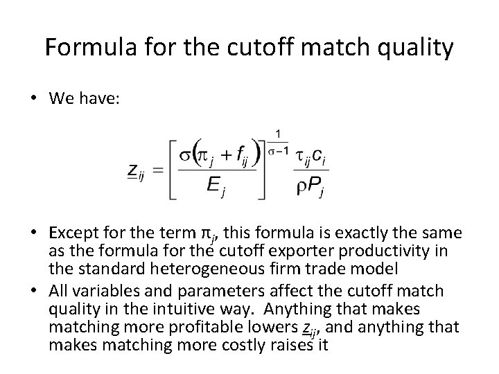
Formula for the cutoff match quality • We have: • Except for the term πj, this formula is exactly the same as the formula for the cutoff exporter productivity in the standard heterogeneous firm trade model • All variables and parameters affect the cutoff match quality in the intuitive way. Anything that makes matching more profitable lowers zij, and anything that makes matching more costly raises it

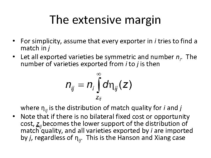
The extensive margin • For simplicity, assume that every exporter in i tries to find a match in j • Let all exported varieties be symmetric and number ni. The number of varieties exported from i to j is then where ηij is the distribution of match quality for i and j • Note that if there is no bilateral fixed cost or opportunity cost, zij becomes the lower support of the distribution of match quality, and all varieties exported by i are imported by j, regardless of ηij. This is the Hanson and Xiang case

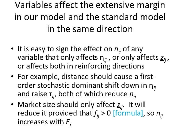
Variables affect the extensive margin in our model and the standard model in the same direction • It is easy to sign the effect on nij of any variable that only affects ηij , or only affects zij , or affects both in reinforcing directions • For example, distance should cause a firstorder stochastic dominant shift down in ηij and raise τij, both of which reduce nij • Market size should only affect zij. It will reduce it provided that fij > 0 [formula], so nij increases with Ej

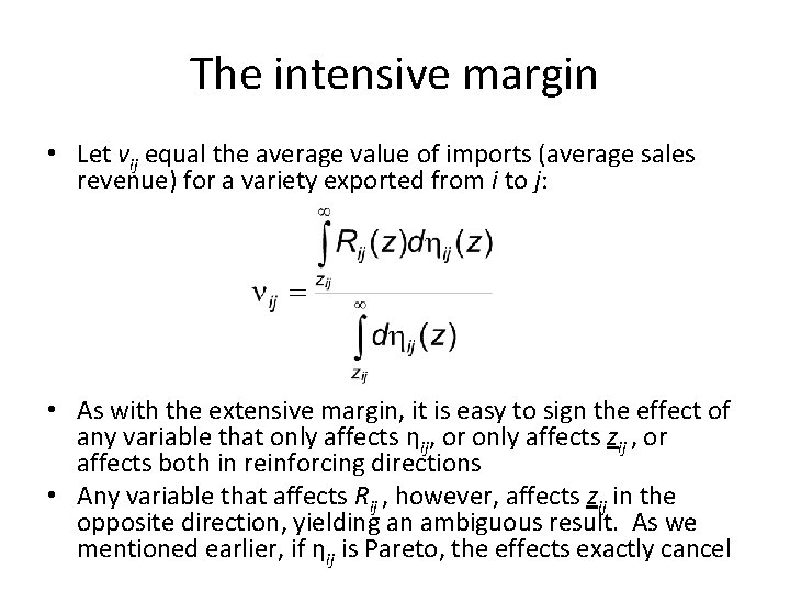
The intensive margin • Let vij equal the average value of imports (average sales revenue) for a variety exported from i to j: • As with the extensive margin, it is easy to sign the effect of any variable that only affects ηij, or only affects zij , or affects both in reinforcing directions • Any variable that affects Rij , however, affects zij in the opposite direction, yielding an ambiguous result. As we mentioned earlier, if ηij is Pareto, the effects exactly cancel

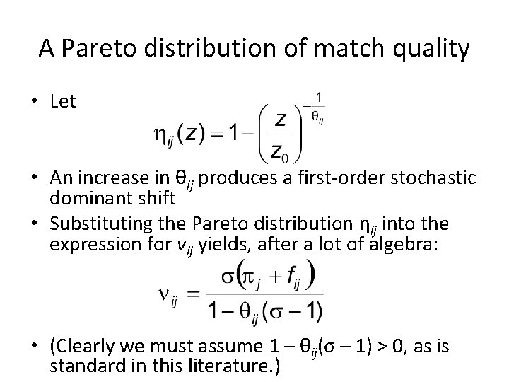
A Pareto distribution of match quality • Let • An increase in θij produces a first-order stochastic dominant shift • Substituting the Pareto distribution ηij into the expression for vij yields, after a lot of algebra: • (Clearly we must assume 1 – θij(σ – 1) > 0, as is standard in this literature. )

Market size, bilateral trade barriers, and the intensive margin • The result that vij is a “markup” over bilateral fixed cost has intuitive appeal. The inclusion of the importer opportunity cost πj in the numerator and the ij subscript on θ are the differences between our model and the standard heterogeneous firm gravity model • Trade barriers that only affect τij do not affect the intensive margin in either model • Because πj increases with market size, the intensive margin increases with market size in our model but not in the standard model • Because bilateral trade barriers can affect fij (the Hanson and Xiang point), only results such as negative effect of distance or positive effect of colonial ties clearly favor our model over the standard model

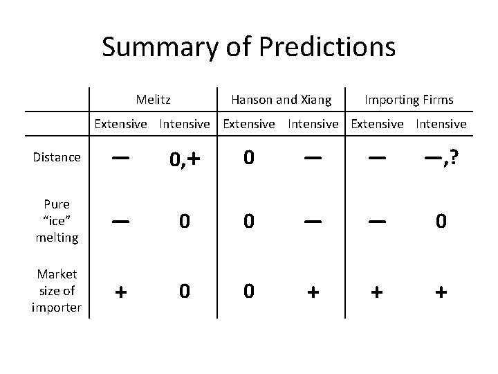
Summary of Predictions Melitz Hanson and Xiang Importing Firms Extensive Intensive Distance — 0, + 0 — — —, ? Pure “ice” melting — 0 0 — — 0 Market size of importer + 0 0 + + +

Conclusions • Our model still needs work. In particular, we have gained much – our theoretical predictions can match the signs of the impacts of market size and trade barriers on both the extensive and intensive margins of bilateral trade – but we have lost log-linearity • Greater scope of distributors (importer-wholesalers or retailers) in economies with larger market sizes is a testable implication of our model • Once again, reducing informational barriers to trade (ηij) has a different impact than reducing “ice” barriers to trade (τij). Both increase bilateral trade in the aggregate and at the extensive margin, but only the former increases trade at the intensive margin