GSEIS LME Logic Synthesis in IC Design and

GSEIS - LME Logic Synthesis in IC Design and Associated Tools Review-II Wang Jiang Chau Grupo de Projeto de Sistemas Eletrônicos e Software Aplicado Laboratório de Microeletrônica – LME Depto. Sistemas Eletrônicos Universidade de São Paulo Escola Politécnica da Universidade de São Paulo

GSEIS - LME Data Structures w Data Type: integer, boolean, etc. Set of values that objects can assume, their common data representation and set of operations on them. Abstract Data Type (ADT): graphs, trees, lists Mathematical model with defined operations Data Structures: arrays, pointers Data types and their relationships, used to implement ADTs Obs. Very common The term Data structure is used to mean ADT Escola Politécnica da Universidade de São Paulo

GSEIS - LME Abstract Data Types (ADTs)- 1 The concept of abstraction means: w We know what a data type can do w How it is done is hidden for the user ØWith an ADT, users are not concerned with how the task is done but rather with what it can do. Escola Politécnica da Universidade de São Paulo

GSEIS - LME Abstract Data Types (ADTs)- 2 w Mathematical model with associated operations. w The implementation is not defined w Two ADTs with the same model, but with different set of operations are considered distinct ones (the implementation may be different depending on the set of operations w Lists, stacks, queues, graphs, trees, heaps Escola Politécnica da Universidade de São Paulo

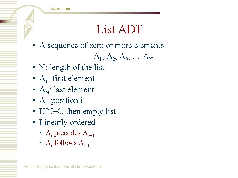
GSEIS - LME List ADT • A sequence of zero or more elements A 1, A 2, A 3, … AN • N: length of the list • A 1: first element • AN: last element • Ai: position i • If N=0, then empty list • Linearly ordered • Ai precedes Ai+1 • Ai follows Ai-1 Escola Politécnica da Universidade de São Paulo

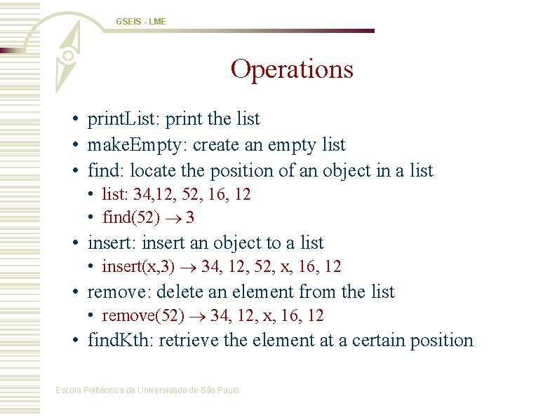
GSEIS - LME Operations • print. List: print the list • make. Empty: create an empty list • find: locate the position of an object in a list • list: 34, 12, 52, 16, 12 • find(52) 3 • insert: insert an object to a list • insert(x, 3) 34, 12, 52, x, 16, 12 • remove: delete an element from the list • remove(52) 34, 12, x, 16, 12 • find. Kth: retrieve the element at a certain position Escola Politécnica da Universidade de São Paulo

GSEIS - LME Implementation of a List • Choose a data structure to represent the list ADT • E. g. arrays, records, etc. • Each operation associated with the list is implemented by one or more subroutines • Two standard implementations for the list ADT • Array-based • Linked list Escola Politécnica da Universidade de São Paulo

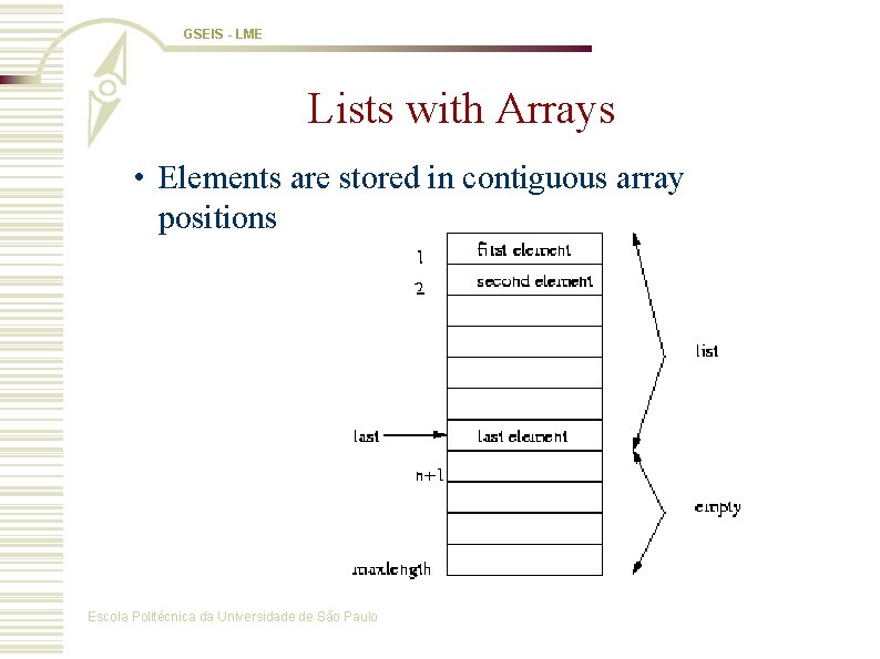
GSEIS - LME Lists with Arrays • Elements are stored in contiguous array positions Escola Politécnica da Universidade de São Paulo

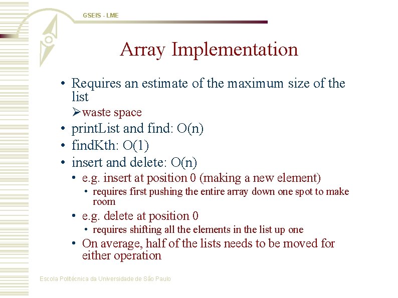
GSEIS - LME Array Implementation • Requires an estimate of the maximum size of the list Ø waste space • print. List and find: O(n) • find. Kth: O(1) • insert and delete: O(n) • e. g. insert at position 0 (making a new element) • requires first pushing the entire array down one spot to make room • e. g. delete at position 0 • requires shifting all the elements in the list up one • On average, half of the lists needs to be moved for either operation Escola Politécnica da Universidade de São Paulo

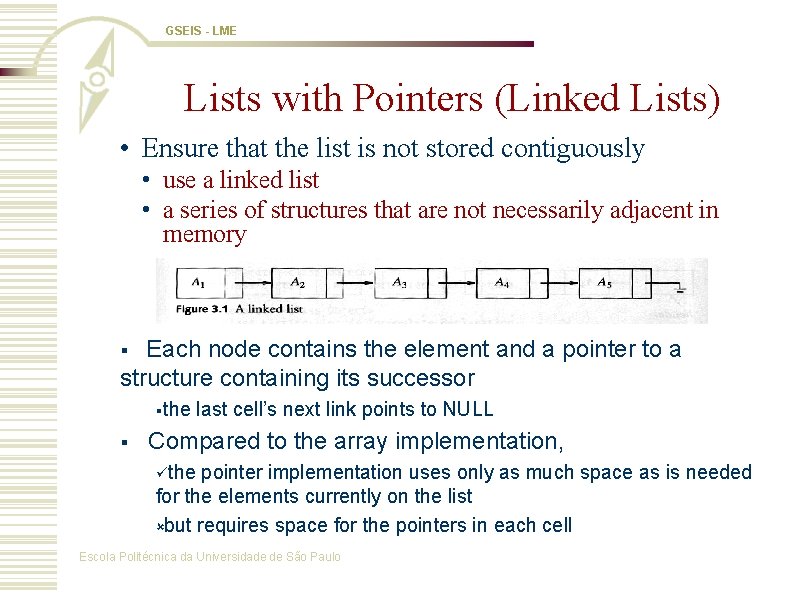
GSEIS - LME Lists with Pointers (Linked Lists) • Ensure that the list is not stored contiguously • use a linked list • a series of structures that are not necessarily adjacent in memory Each node contains the element and a pointer to a structure containing its successor § §the § last cell’s next link points to NULL Compared to the array implementation, üthe pointer implementation uses only as much space as is needed for the elements currently on the list ûbut requires space for the pointers in each cell Escola Politécnica da Universidade de São Paulo

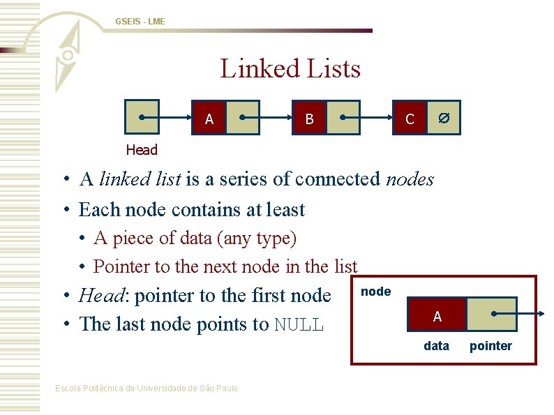
GSEIS - LME Linked Lists A B C Head • A linked list is a series of connected nodes • Each node contains at least • A piece of data (any type) • Pointer to the next node in the list • Head: pointer to the first node • The last node points to NULL node A data Escola Politécnica da Universidade de São Paulo pointer

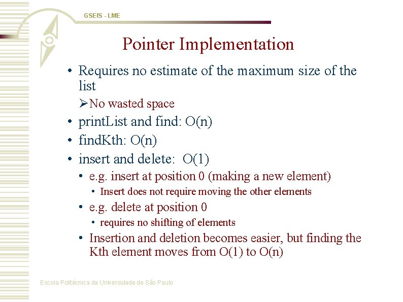
GSEIS - LME Pointer Implementation • Requires no estimate of the maximum size of the list Ø No wasted space • print. List and find: O(n) • find. Kth: O(n) • insert and delete: O(1) • e. g. insert at position 0 (making a new element) • Insert does not require moving the other elements • e. g. delete at position 0 • requires no shifting of elements • Insertion and deletion becomes easier, but finding the Kth element moves from O(1) to O(n) Escola Politécnica da Universidade de São Paulo

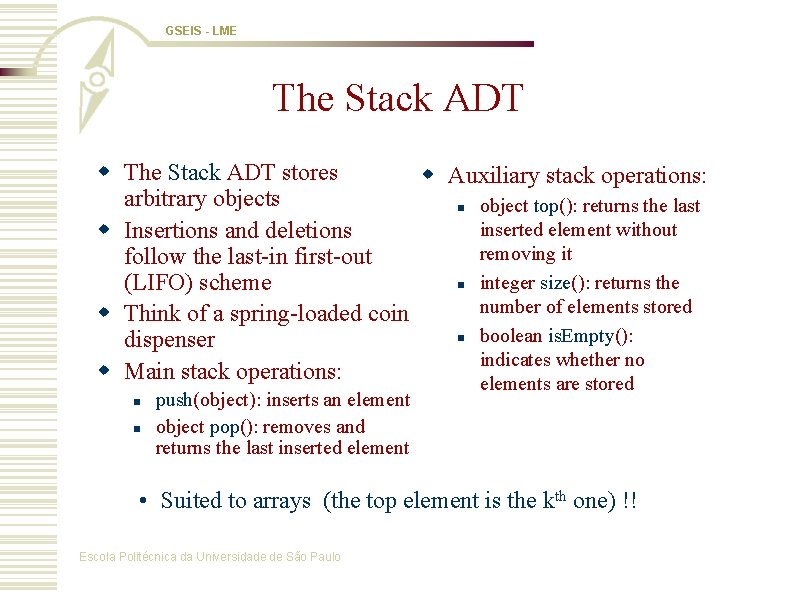
GSEIS - LME The Stack ADT w The Stack ADT stores w Auxiliary stack operations: arbitrary objects n object top(): returns the last inserted element without w Insertions and deletions removing it follow the last-in first-out n integer size(): returns the (LIFO) scheme number of elements stored w Think of a spring-loaded coin n boolean is. Empty(): dispenser indicates whether no w Main stack operations: elements are stored n n push(object): inserts an element object pop(): removes and returns the last inserted element • Suited to arrays (the top element is the kth one) !! Escola Politécnica da Universidade de São Paulo

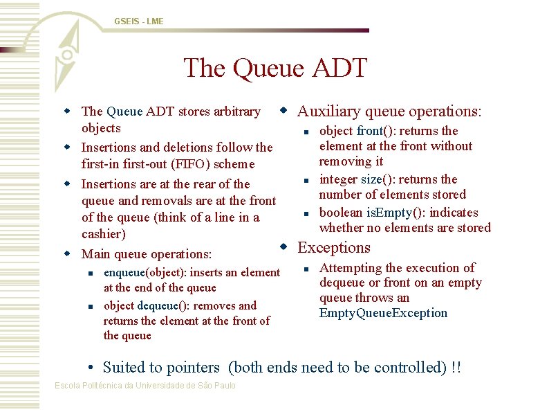
GSEIS - LME The Queue ADT w The Queue ADT stores arbitrary w Auxiliary queue operations: objects n object front(): returns the element at the front without w Insertions and deletions follow the removing it first-in first-out (FIFO) scheme n integer size(): returns the w Insertions are at the rear of the number of elements stored queue and removals are at the front n boolean is. Empty(): indicates of the queue (think of a line in a whether no elements are stored cashier) w Exceptions w Main queue operations: n Attempting the execution of n enqueue(object): inserts an element dequeue or front on an empty at the end of the queue throws an n object dequeue(): removes and Empty. Queue. Exception returns the element at the front of the queue • Suited to pointers (both ends need to be controlled) !! Escola Politécnica da Universidade de São Paulo

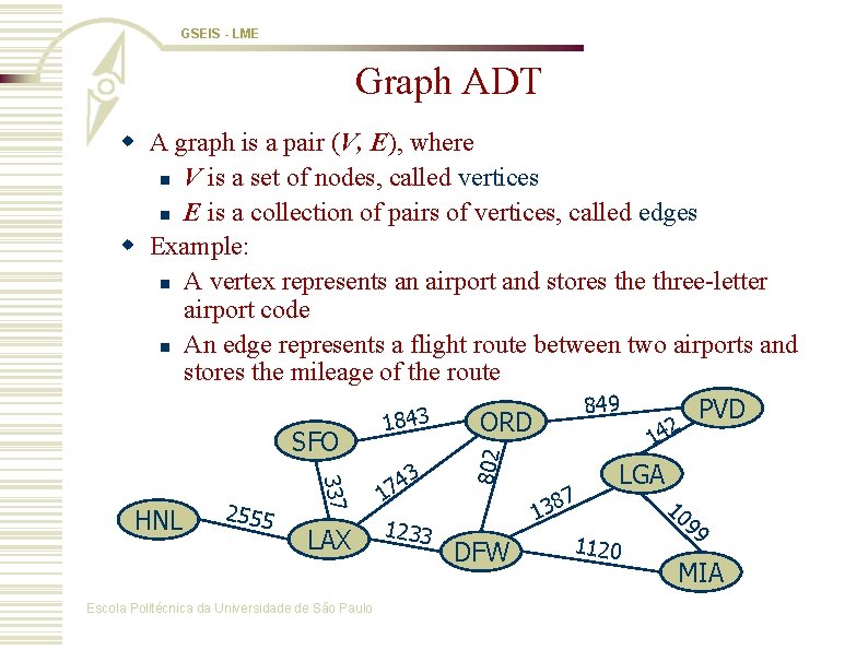
GSEIS - LME Graph ADT HNL 2555 LAX Escola Politécnica da Universidade de São Paulo 1 1233 802 337 w A graph is a pair (V, E), where n V is a set of nodes, called vertices n E is a collection of pairs of vertices, called edges w Example: n A vertex represents an airport and stores the three-letter airport code n An edge represents a flight route between two airports and stores the mileage of the route 849 PVD 3 4 ORD 18 2 4 1 SFO 3 LGA 74 DFW 7 8 3 1 1120 10 99 MIA

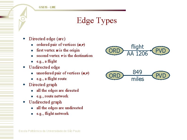
GSEIS - LME Edge Types w Directed edge (arc) n n ordered pair of vertices (u, v) first vertex u is the origin second vertex v is the destination e. g. , a flight ORD flight AA 1206 PVD ORD 849 miles PVD w Undirected edge n n unordered pair of vertices (u, v) e. g. , a flight route w Directed graph n n all the edges are directed e. g. , route network w Undirected graph n n all the edges are undirected e. g. , flight network Escola Politécnica da Universidade de São Paulo

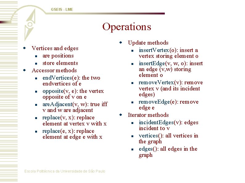
GSEIS - LME Operations w Vertices and edges n are positions n store elements w Accessor methods n end. Vertices(e): the two endvertices of e n opposite(v, e): the vertex opposite of v on e n are. Adjacent(v, w): true iff v and w are adjacent n replace(v, x): replace element at vertex v with x n replace(e, x): replace element at edge e with x Escola Politécnica da Universidade de São Paulo w Update methods n insert. Vertex(o): insert a vertex storing element o n insert. Edge(v, w, o): insert an edge (v, w) storing element o n remove. Vertex(v): remove vertex v (and its incident edges) n remove. Edge(e): remove edge e w Iterator methods n incident. Edges(v): edges incident to v n vertices(): all vertices in the graph n edges(): all edges in the graph

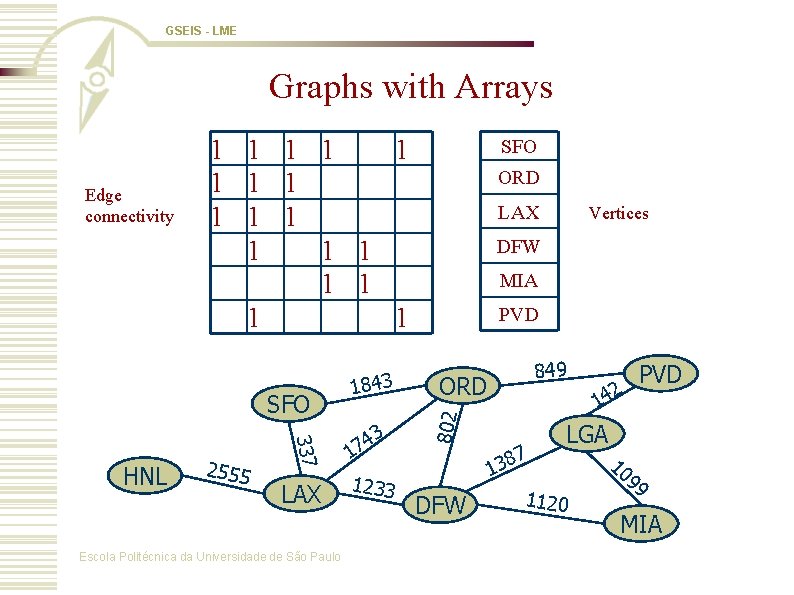
GSEIS - LME Graphs with Arrays SFO 337 HNL 2555 LAX Escola Politécnica da Universidade de São Paulo 1843 3 4 7 1 1233 SFO ORD LAX Vertices DFW MIA PVD 849 ORD 802 Edge connectivity 1 1 1 1 1 DFW 2 PVD 14 7 8 3 1 LGA 1120 10 99 MIA

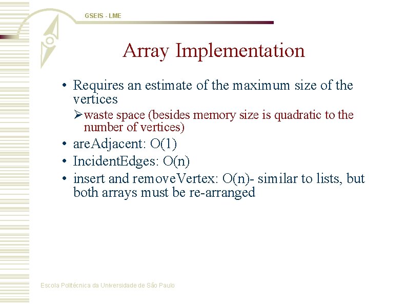
GSEIS - LME Array Implementation • Requires an estimate of the maximum size of the vertices Ø waste space (besides memory size is quadratic to the number of vertices) • are. Adjacent: O(1) • Incident. Edges: O(n) • insert and remove. Vertex: O(n)- similar to lists, but both arrays must be re-arranged Escola Politécnica da Universidade de São Paulo

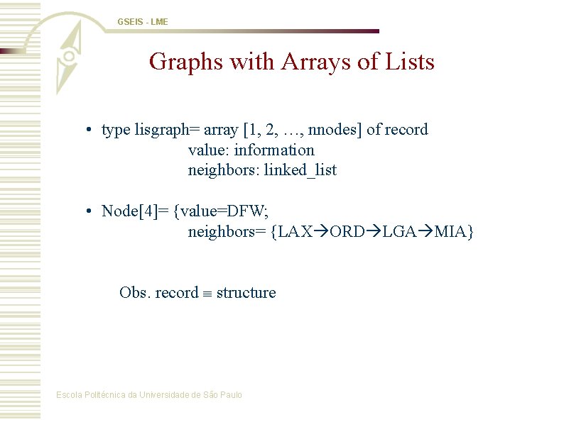
GSEIS - LME Graphs with Arrays of Lists • type lisgraph= array [1, 2, …, nnodes] of record value: information neighbors: linked_list • Node[4]= {value=DFW; neighbors= {LAX ORD LGA MIA} Obs. record structure Escola Politécnica da Universidade de São Paulo

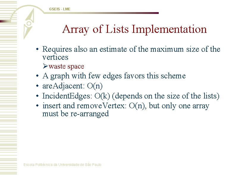
GSEIS - LME Array of Lists Implementation • Requires also an estimate of the maximum size of the vertices Ø waste space • • A graph with few edges favors this scheme are. Adjacent: O(n) Incident. Edges: O(k) (depends on the size of the lists) insert and remove. Vertex: O(n), but only one array must be re-arranged Escola Politécnica da Universidade de São Paulo

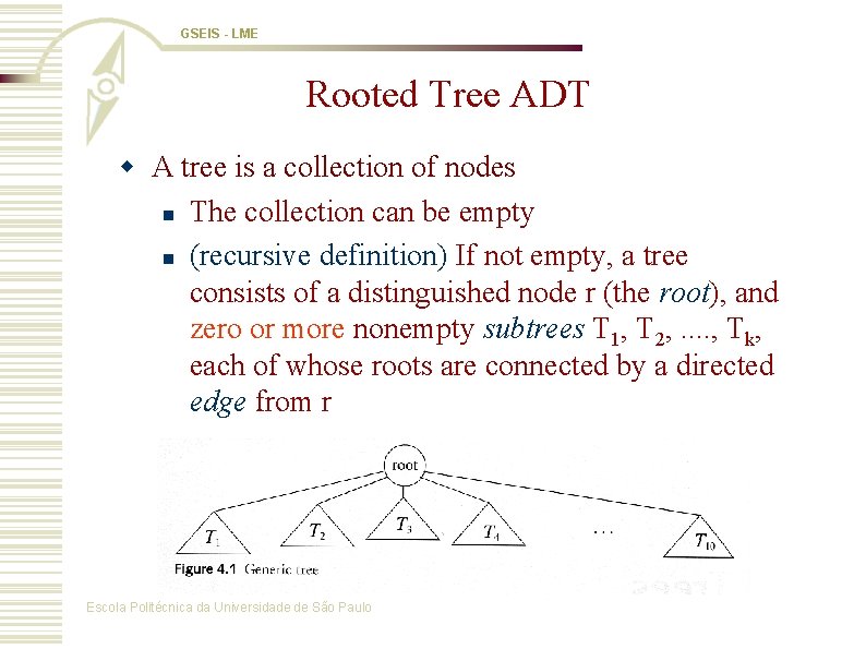
GSEIS - LME Rooted Tree ADT w A tree is a collection of nodes n The collection can be empty n (recursive definition) If not empty, a tree consists of a distinguished node r (the root), and zero or more nonempty subtrees T 1, T 2, . . , Tk, each of whose roots are connected by a directed edge from r Escola Politécnica da Universidade de São Paulo

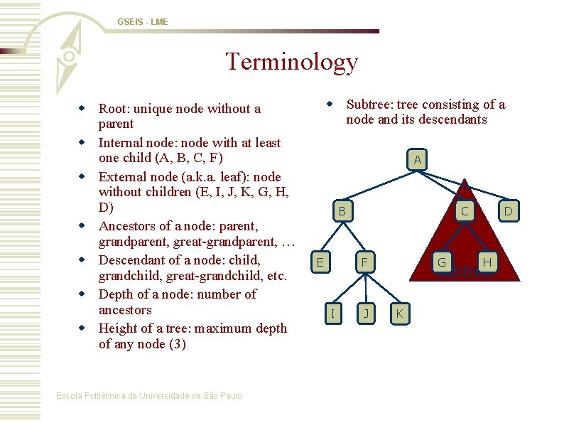
GSEIS - LME Terminology w Root: unique node without a parent w Internal node: node with at least one child (A, B, C, F) w External node (a. k. a. leaf): node without children (E, I, J, K, G, H, D) w Ancestors of a node: parent, grandparent, great-grandparent, … w Descendant of a node: child, grandchild, great-grandchild, etc. w Depth of a node: number of ancestors w Height of a tree: maximum depth of any node (3) Escola Politécnica da Universidade de São Paulo w Subtree: tree consisting of a node and its descendants A B E C F I J G D H subtree K

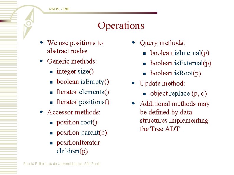
GSEIS - LME Operations w We use positions to abstract nodes w Generic methods: n integer size() n boolean is. Empty() n Iterator elements() n Iterator positions() w Accessor methods: n position root() n position parent(p) n position. Iterator children(p) Escola Politécnica da Universidade de São Paulo w Query methods: n boolean is. Internal(p) n boolean is. External(p) n boolean is. Root(p) w Update method: n object replace (p, o) w Additional methods may be defined by data structures implementing the Tree ADT

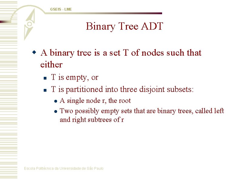
GSEIS - LME Binary Tree ADT w A binary tree is a set T of nodes such that either n n T is empty, or T is partitioned into three disjoint subsets: l l A single node r, the root Two possibly empty sets that are binary trees, called left and right subtrees of r Escola Politécnica da Universidade de São Paulo

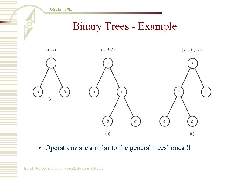
GSEIS - LME Binary Trees - Example • Operations are similar to the general trees’ ones !! Escola Politécnica da Universidade de São Paulo

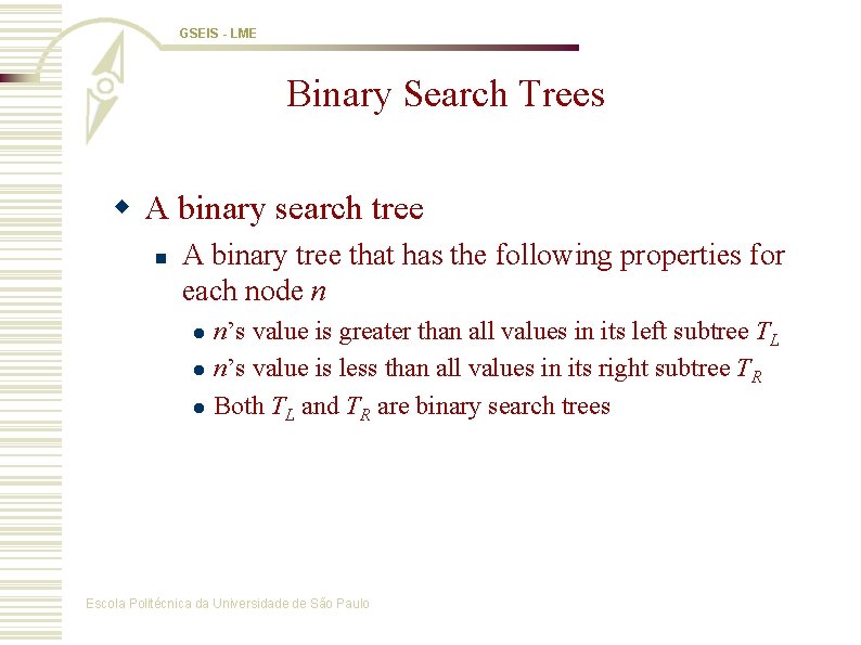
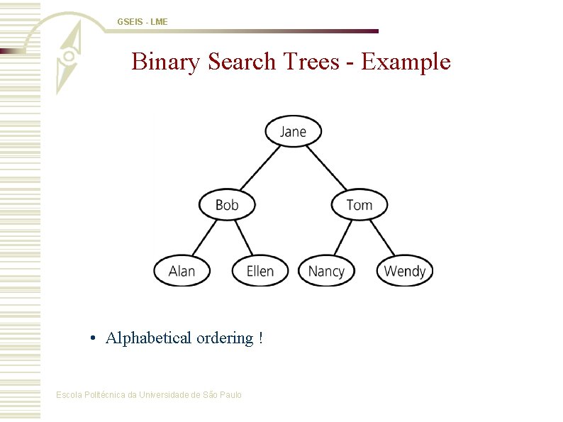
GSEIS - LME Binary Search Trees w A binary search tree n A binary tree that has the following properties for each node n l l l n’s value is greater than all values in its left subtree TL n’s value is less than all values in its right subtree TR Both TL and TR are binary search trees Escola Politécnica da Universidade de São Paulo

GSEIS - LME Binary Search Trees - Example • Alphabetical ordering ! Escola Politécnica da Universidade de São Paulo

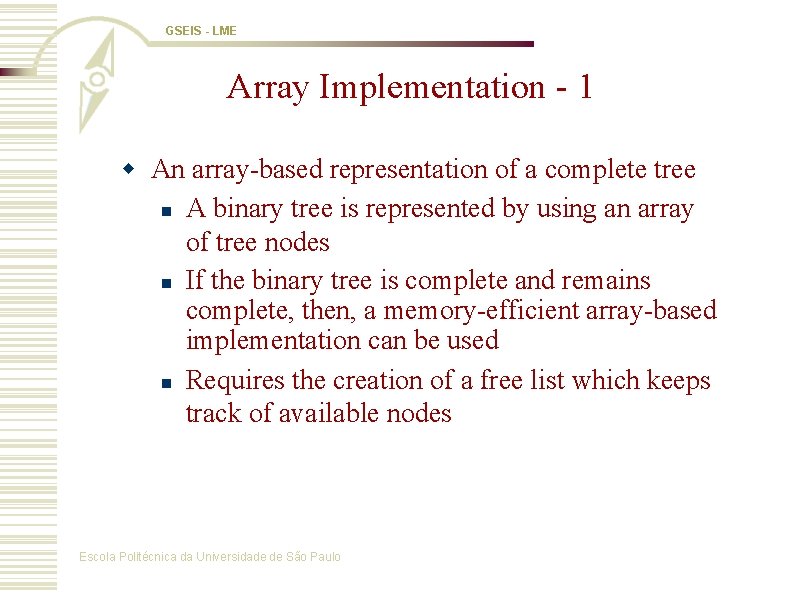
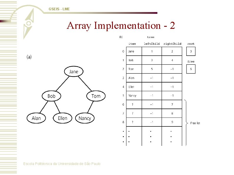
GSEIS - LME Array Implementation - 1 w An array-based representation of a complete tree n A binary tree is represented by using an array of tree nodes n If the binary tree is complete and remains complete, then, a memory-efficient array-based implementation can be used n Requires the creation of a free list which keeps track of available nodes Escola Politécnica da Universidade de São Paulo

GSEIS - LME Array Implementation - 2 Escola Politécnica da Universidade de São Paulo

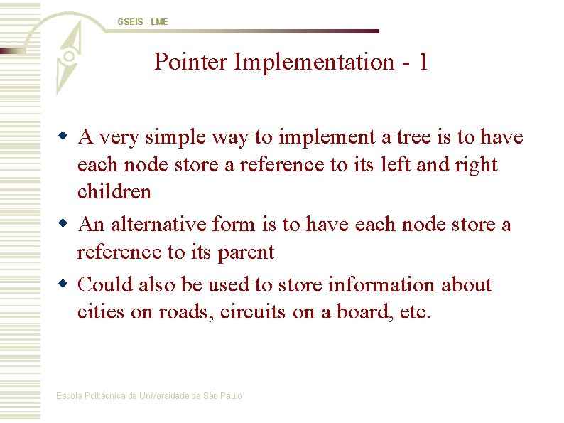
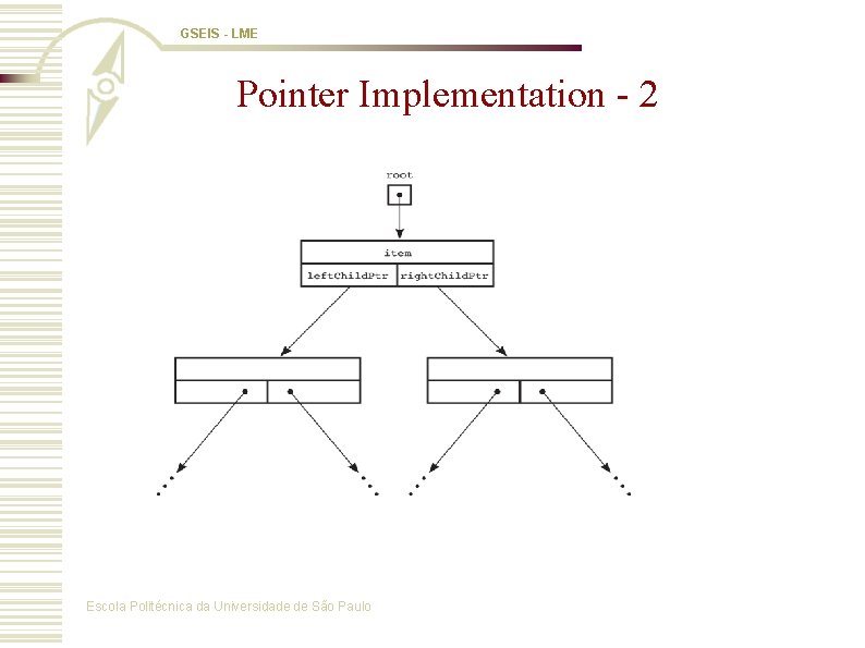
GSEIS - LME Pointer Implementation - 1 w A very simple way to implement a tree is to have each node store a reference to its left and right children w An alternative form is to have each node store a reference to its parent w Could also be used to store information about cities on roads, circuits on a board, etc. Escola Politécnica da Universidade de São Paulo

GSEIS - LME Pointer Implementation - 2 Escola Politécnica da Universidade de São Paulo

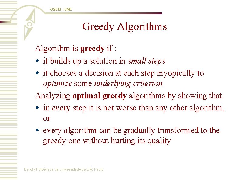
GSEIS - LME Greedy Algorithms Algorithm is greedy if : w it builds up a solution in small steps w it chooses a decision at each step myopically to optimize some underlying criterion Analyzing optimal greedy algorithms by showing that: w in every step it is not worse than any other algorithm, or w every algorithm can be gradually transformed to the greedy one without hurting its quality Escola Politécnica da Universidade de São Paulo

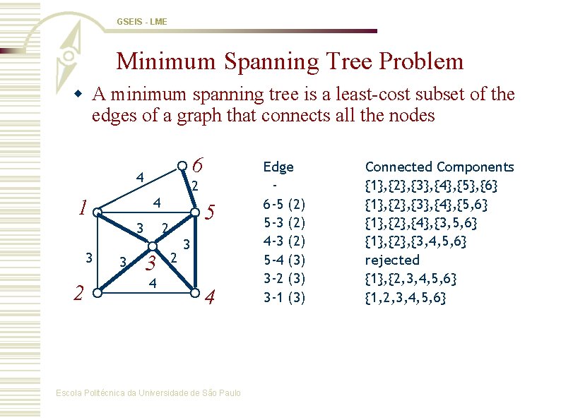
GSEIS - LME Minimum Spanning Tree Problem w A minimum spanning tree is a least-cost subset of the edges of a graph that connects all the nodes 6 4 2 4 1 3 3 2 3 5 2 3 4 Escola Politécnica da Universidade de São Paulo Edge 6 -5 (2) 5 -3 (2) 4 -3 (2) 5 -4 (3) 3 -2 (3) 3 -1 (3) Connected Components {1}, {2}, {3}, {4}, {5}, {6} {1}, {2}, {3}, {4}, {5, 6} {1}, {2}, {4}, {3, 5, 6} {1}, {2}, {3, 4, 5, 6} rejected {1}, {2, 3, 4, 5, 6} {1, 2, 3, 4, 5, 6}

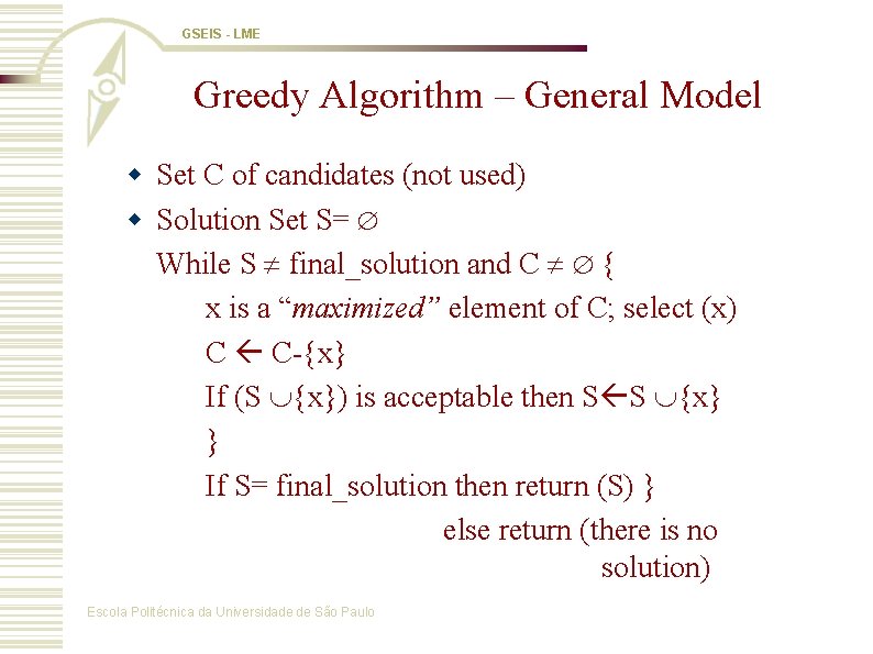
GSEIS - LME Greedy Algorithm – General Model w Set C of candidates (not used) w Solution Set S= While S final_solution and C { x is a “maximized” element of C; select (x) C C-{x} If (S {x}) is acceptable then S S {x} } If S= final_solution then return (S) } else return (there is no solution) Escola Politécnica da Universidade de São Paulo

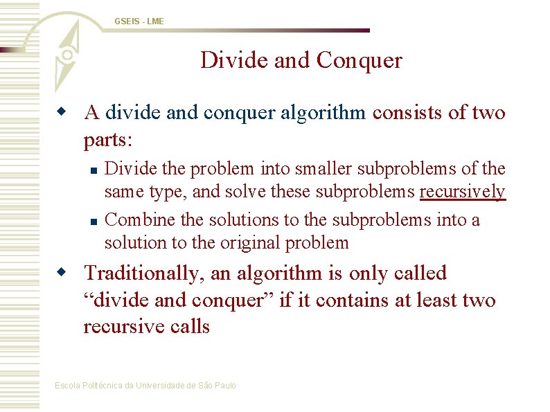
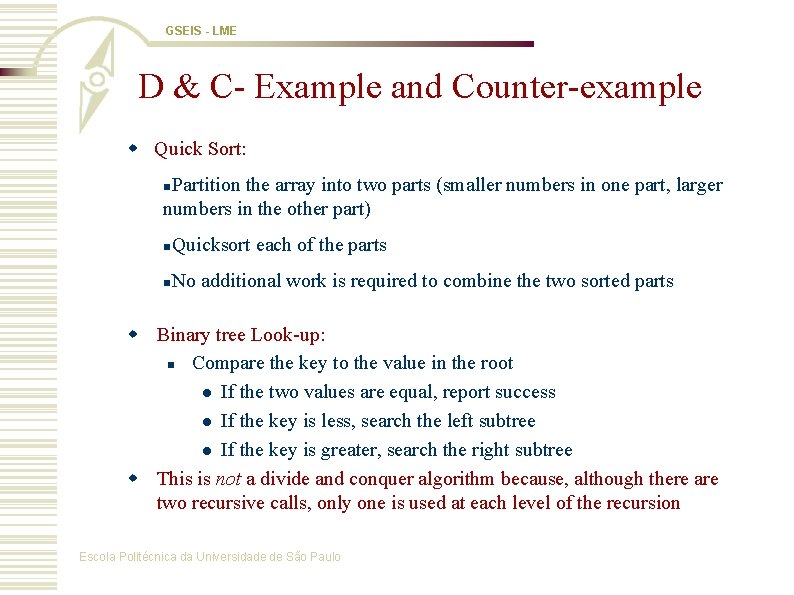
GSEIS - LME Divide and Conquer w A divide and conquer algorithm consists of two parts: n n Divide the problem into smaller subproblems of the same type, and solve these subproblems recursively Combine the solutions to the subproblems into a solution to the original problem w Traditionally, an algorithm is only called “divide and conquer” if it contains at least two recursive calls Escola Politécnica da Universidade de São Paulo

GSEIS - LME D & C- Example and Counter-example w Quick Sort: Partition the array into two parts (smaller numbers in one part, larger numbers in the other part) n n Quicksort each of the parts n No additional work is required to combine the two sorted parts w Binary tree Look-up: n Compare the key to the value in the root l If the two values are equal, report success l If the key is less, search the left subtree l If the key is greater, search the right subtree w This is not a divide and conquer algorithm because, although there are two recursive calls, only one is used at each level of the recursion Escola Politécnica da Universidade de São Paulo

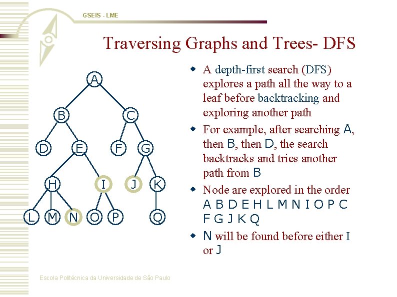
GSEIS - LME Traversing Graphs and Trees- DFS A B D C E H L M N O F I G J P K Q Escola Politécnica da Universidade de São Paulo w A depth-first search (DFS) explores a path all the way to a leaf before backtracking and exploring another path w For example, after searching A, then B, then D, the search backtracks and tries another path from B w Node are explored in the order ABDEHLMNIOPC FGJKQ w N will be found before either I or J

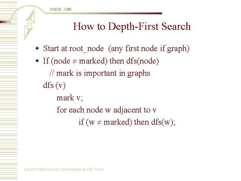
GSEIS - LME How to Depth-First Search w Start at root_node (any first node if graph) w If (node marked) then dfs(node) // mark is important in graphs dfs (v) mark v; for each node w adjacent to v if (w marked) then dfs(w); Escola Politécnica da Universidade de São Paulo

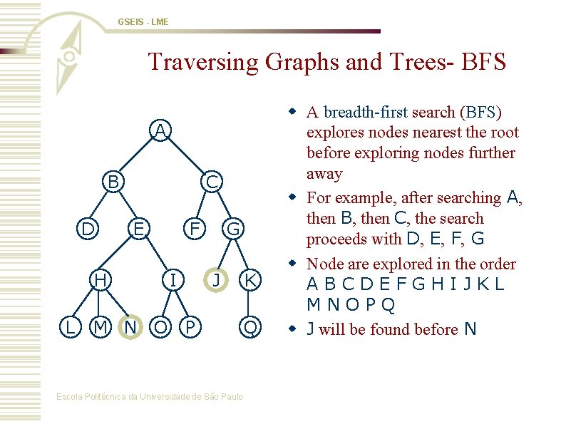
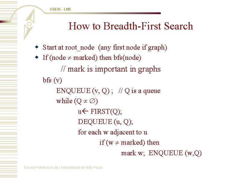
GSEIS - LME Traversing Graphs and Trees- BFS A B D C E H L M N O F I G J P Escola Politécnica da Universidade de São Paulo K Q w A breadth-first search (BFS) explores nodes nearest the root before exploring nodes further away w For example, after searching A, then B, then C, the search proceeds with D, E, F, G w Node are explored in the order ABCDEFGHIJKL MNOPQ w J will be found before N

GSEIS - LME How to Breadth-First Search w Start at root_node (any first node if graph) w If (node marked) then bfs(node) // mark is important in graphs bfs (v) ENQUEUE (v, Q) ; // Q is a queue while (Q ) u FIRST(Q); DEQUEUE (u, Q); for each w adjacent to u if (w marked) then mark w; ENQUEUE (w, Q) Escola Politécnica da Universidade de São Paulo

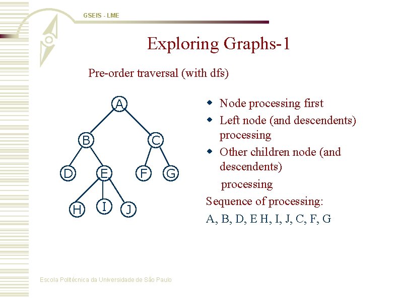
GSEIS - LME Exploring Graphs-1 Pre-order traversal (with dfs) A B D H C E I F G J Escola Politécnica da Universidade de São Paulo w Node processing first w Left node (and descendents) processing w Other children node (and descendents) processing Sequence of processing: A, B, D, E H, I, J, C, F, G

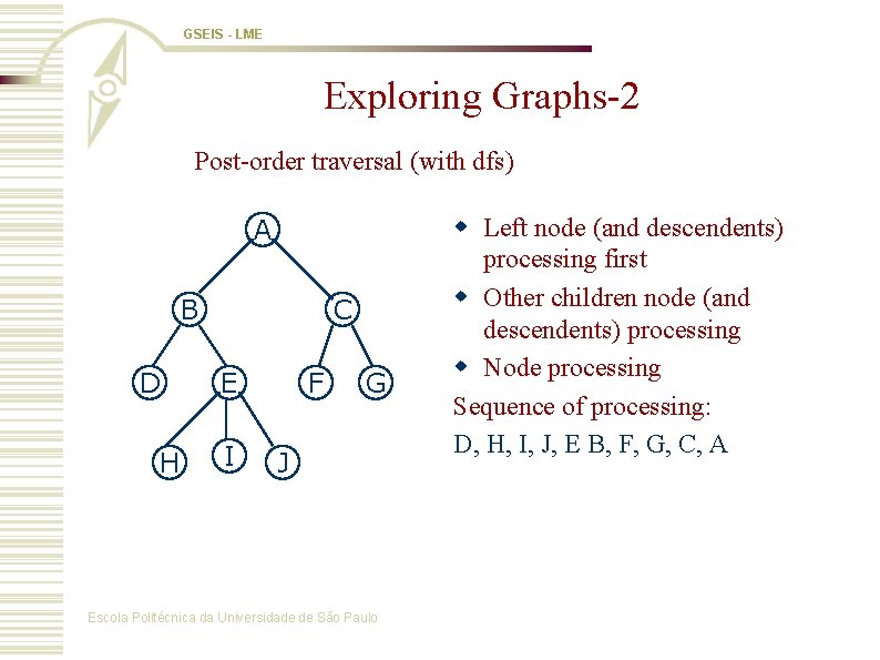
GSEIS - LME Exploring Graphs-2 Post-order traversal (with dfs) A B D H C E I F G J Escola Politécnica da Universidade de São Paulo w Left node (and descendents) processing first w Other children node (and descendents) processing w Node processing Sequence of processing: D, H, I, J, E B, F, G, C, A

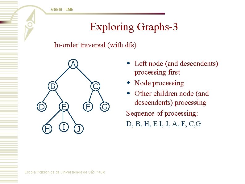
GSEIS - LME Exploring Graphs-3 In-order traversal (with dfs) A B D H C E I F G J Escola Politécnica da Universidade de São Paulo w Left node (and descendents) processing first w Node processing w Other children node (and descendents) processing Sequence of processing: D, B, H, E I, J, A, F, C, G

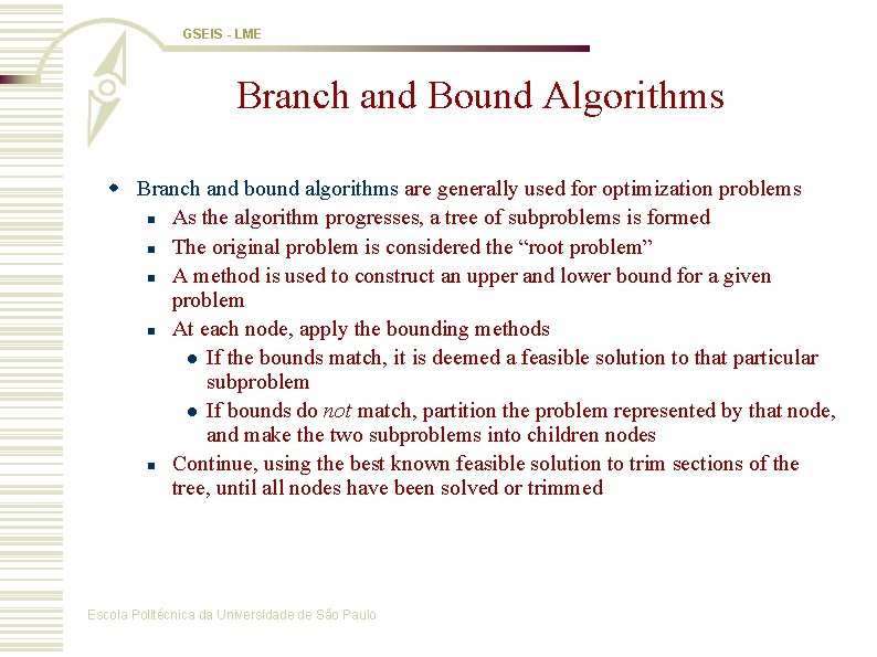
GSEIS - LME Branch and Bound Algorithms w Branch and bound algorithms are generally used for optimization problems n As the algorithm progresses, a tree of subproblems is formed n The original problem is considered the “root problem” n A method is used to construct an upper and lower bound for a given problem n At each node, apply the bounding methods l If the bounds match, it is deemed a feasible solution to that particular subproblem l If bounds do not match, partition the problem represented by that node, and make the two subproblems into children nodes n Continue, using the best known feasible solution to trim sections of the tree, until all nodes have been solved or trimmed Escola Politécnica da Universidade de São Paulo

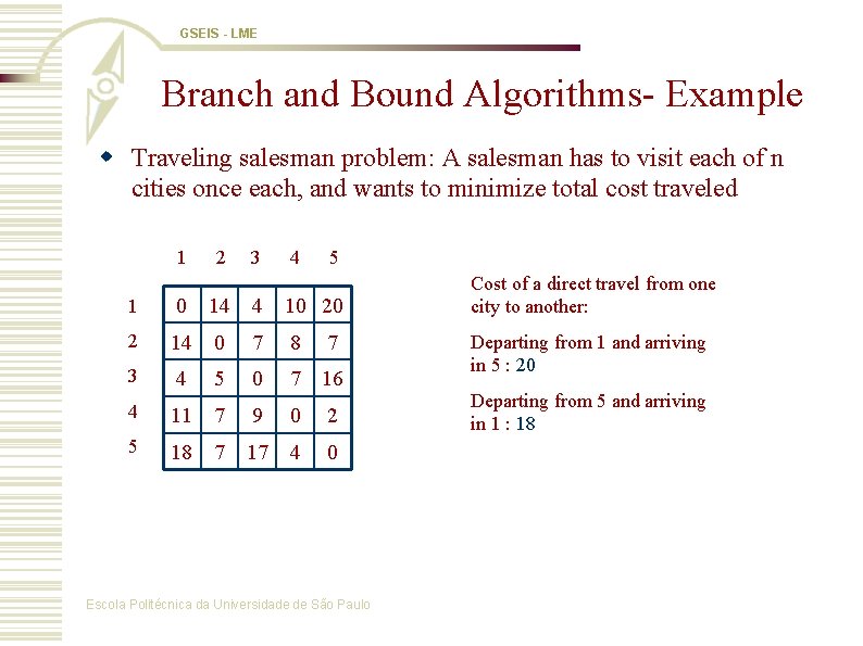
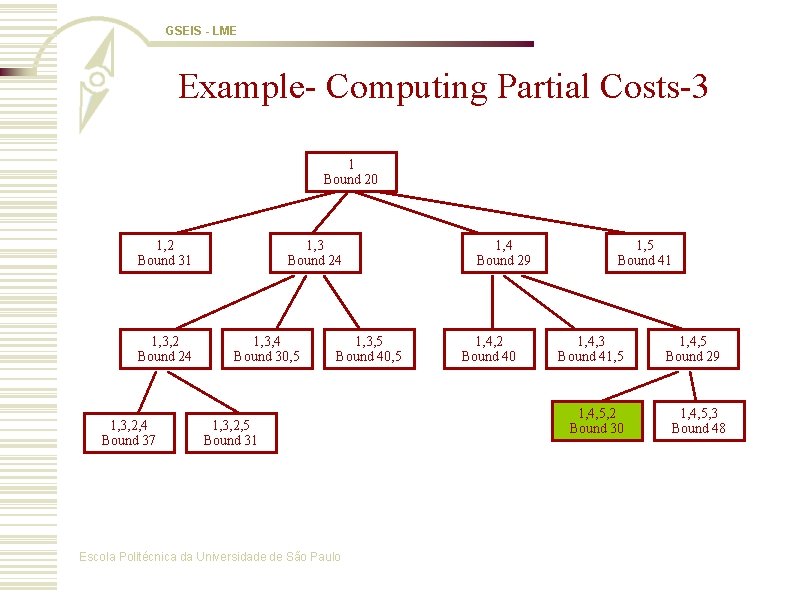
GSEIS - LME Branch and Bound Algorithms- Example w Traveling salesman problem: A salesman has to visit each of n cities once each, and wants to minimize total cost traveled 1 2 3 4 5 1 0 14 4 10 20 2 14 0 7 8 3 4 5 0 7 16 4 11 7 9 0 2 5 18 7 17 4 0 7 Escola Politécnica da Universidade de São Paulo Cost of a direct travel from one city to another: Departing from 1 and arriving in 5 : 20 Departing from 5 and arriving in 1 : 18

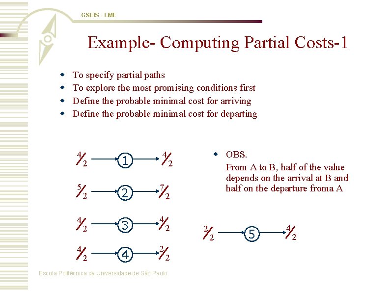
GSEIS - LME Example- Computing Partial Costs-1 w w To specify partial paths To explore the most promising conditions first Define the probable minimal cost for arriving Define the probable minimal cost for departing 4 5 4 4 4 2 1 2 2 7 3 4 2 2 4 2 w OBS. From A to B, half of the value depends on the arrival at B and half on the departure froma A 2 2 Escola Politécnica da Universidade de São Paulo 2 2 5 4 2

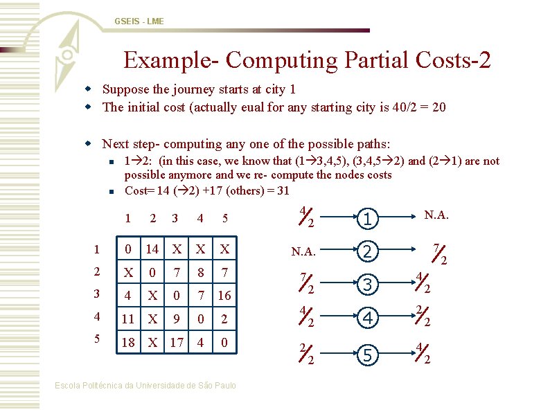
GSEIS - LME Example- Computing Partial Costs-2 w Suppose the journey starts at city 1 w The initial cost (actually eual for any starting city is 40/2 = 20 w Next step- computing any one of the possible paths: n n 1 2: (in this case, we know that (1 3, 4, 5), (3, 4, 5 2) and (2 1) are not possible anymore and we re- compute the nodes costs Cost= 14 ( 2) +17 (others) = 31 1 2 4 2 1 N. A. X N. A. 2 7 7 7 3 4 5 1 0 14 X X 2 X 0 7 8 3 4 X 0 7 16 4 11 X 9 0 2 5 18 X 17 4 0 Escola Politécnica da Universidade de São Paulo 4 2 2 3 4 4 2 5 4 2 2

GSEIS - LME Example- Computing Partial Costs-3 1 Bound 20 1, 2 Bound 31 1, 3, 2 Bound 24 1, 3, 2, 4 Bound 37 1, 3 Bound 24 1, 3, 4 Bound 30, 5 1, 3, 5 Bound 40, 5 1, 3, 2, 5 Bound 31 Escola Politécnica da Universidade de São Paulo 1, 4 Bound 29 1, 4, 2 Bound 40 1, 5 Bound 41 1, 4, 3 Bound 41, 5 1, 4, 5, 2 Bound 30 1, 4, 5 Bound 29 1, 4, 5, 3 Bound 48