LME 4 Andrea Friese Silvia Artuso Danai Laina

LME 4 Andrea Friese, Silvia Artuso, Danai Laina

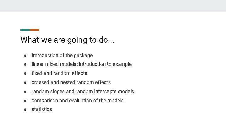
What we are going to do. . . ● introduction of the package ● linear mixed models: introduction to example ● fixed and random effects ● crossed and nested random effects ● random slopes and random intercepts models ● comparison and evaluation of the models ● statistics

About lme 4 ● provides functions to fit and analyze statistical linear mixed models, generalized mixed models, and nonlinear mixed models ● we focus on linear mixed models ● what they are? → I’ll get there

● mainly used in fields like biology, physics, or social sciences ● developed by Bates, Mächler, Bolker and Walker around 2012 ● fundamentally based on its predecessor nlme ● lme 4 as baseline for multilevel models + various packages that enhance its feature set

Now: what is a linear mixed model? ● picture a basic linear model with one dependent variable and one independent variable ( = fixed effect) ● add various fixed effects ● add random effects ● random effect: a factor we want to control, because it can affect the result; “grouping-factor”

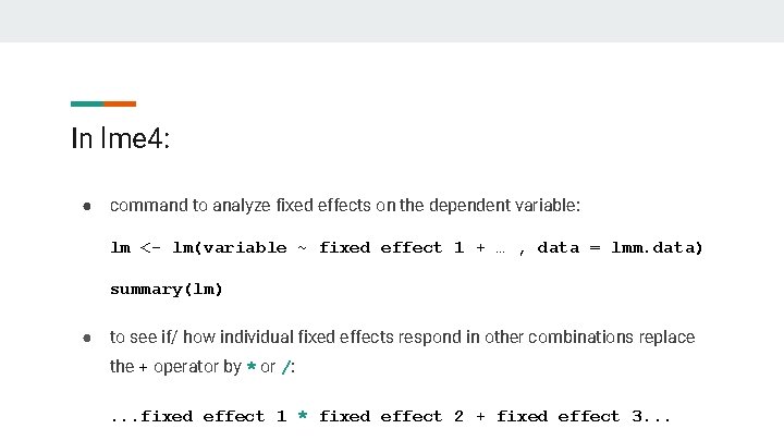
In lme 4: ● command to analyze fixed effects on the dependent variable: lm <- lm(variable ~ fixed effect 1 + … , data = lmm. data) summary(lm) ● to see if/ how individual fixed effects respond in other combinations replace the + operator by * or /: . . . fixed effect 1 * fixed effect 2 + fixed effect 3. . .

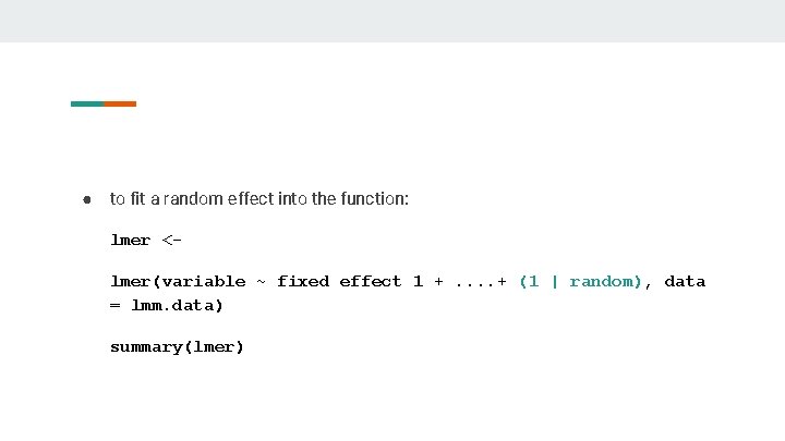
● to fit a random effect into the function: lmer <lmer(variable ~ fixed effect 1 +. . + (1 | random), data = lmm. data) summary(lmer)

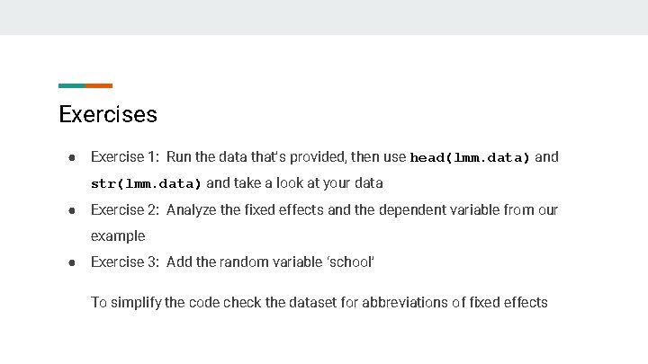
Exercises ● Exercise 1: Run the data that’s provided, then use head(lmm. data) and str(lmm. data) and take a look at your data ● Exercise 2: Analyze the fixed effects and the dependent variable from our example ● Exercise 3: Add the random variable ‘school’ To simplify the code check the dataset for abbreviations of fixed effects

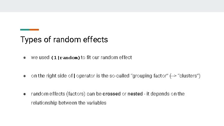
Types of random effects ● we used (1|random)to fit our random effect ● on the right side of | operator is the so-called “grouping factor” (--> “clusters”) ● random effects (factors) can be crossed or nested - it depends on the relationship between the variables

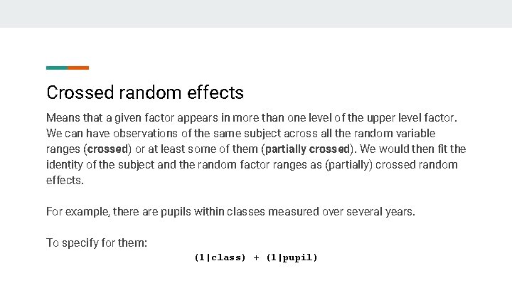
Crossed random effects Means that a given factor appears in more than one level of the upper level factor. We can have observations of the same subject across all the random variable ranges (crossed) or at least some of them (partially crossed). We would then fit the identity of the subject and the random factor ranges as (partially) crossed random effects. For example, there are pupils within classes measured over several years. To specify for them: (1|class) + (1|pupil)

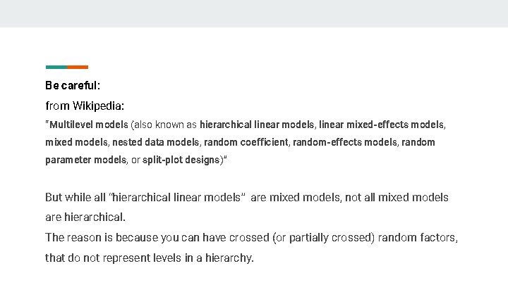
Be careful: from Wikipedia: “Multilevel models (also known as hierarchical linear models, linear mixed-effects models, mixed models, nested data models, random coefficient, random-effects models, random parameter models, or split-plot designs)” But while all “hierarchical linear models” are mixed models, not all mixed models are hierarchical. The reason is because you can have crossed (or partially crossed) random factors, that do not represent levels in a hierarchy.

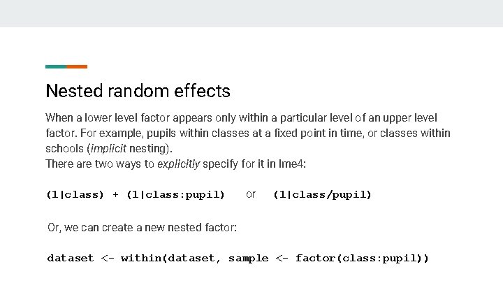
Nested random effects When a lower level factor appears only within a particular level of an upper level factor. For example, pupils within classes at a fixed point in time, or classes within schools (implicit nesting). There are two ways to explicitly specify for it in lme 4: (1|class) + (1|class: pupil) or (1|class/pupil) Or, we can create a new nested factor: dataset <- within(dataset, sample <- factor(class: pupil))

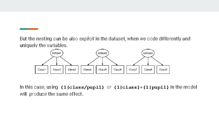
But the nesting can be also explicit in the dataset, when we code differently and uniquely the variables. In this case, using (1|class/pupil) or (1|class)+(1|pupil) in the model will produce the same effect.

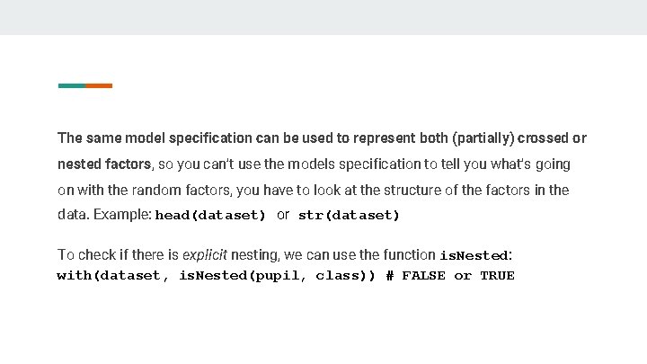
The same model specification can be used to represent both (partially) crossed or nested factors, so you can’t use the models specification to tell you what’s going on with the random factors, you have to look at the structure of the factors in the data. Example: head(dataset) or str(dataset) To check if there is explicit nesting, we can use the function is. Nested: with(dataset, is. Nested(pupil, class)) # FALSE or TRUE

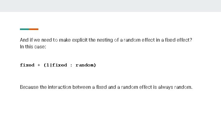
And if we need to make explicit the nesting of a random effect in a fixed effect? In this case: fixed + (1|fixed : random) Because the interaction between a fixed and a random effect is always random.

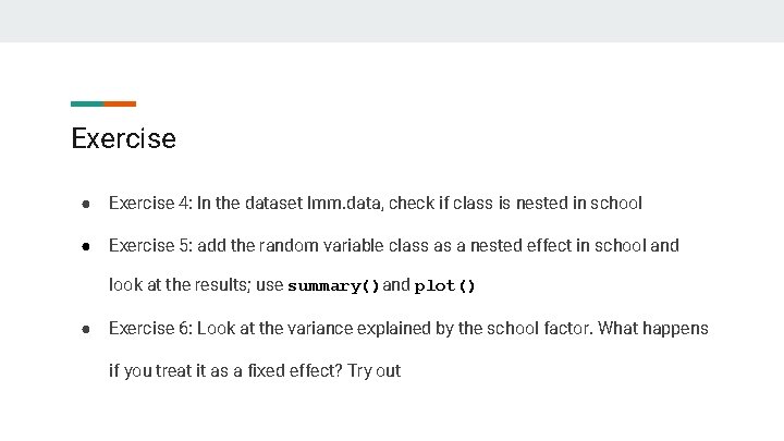
Exercise ● Exercise 4: In the dataset lmm. data, check if class is nested in school ● Exercise 5: add the random variable class as a nested effect in school and look at the results; use summary()and plot() ● Exercise 6: Look at the variance explained by the school factor. What happens if you treat it as a fixed effect? Try out

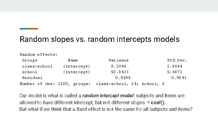
Random slopes vs. random intercepts models Random effects: Groups Name class: school (Intercept) Residual Number of obs: 1200, groups: Variance Std. Dev. 8. 2046 2. 8644 93. 8433 9. 6873 0. 9684 0. 9841 class: school, 24; school, 6 Our model is what is called a random intercept model: subjects and items are allowed to have different intercept, but not different slopes → coef(). But what if we think that a fixed effect is not the same for all subjects and items?

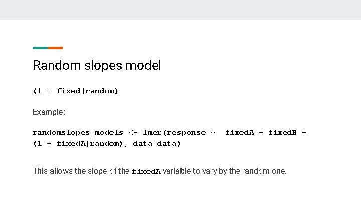
Random slopes model (1 + fixed|random) Example: randomslopes_models <- lmer(response ~ (1 + fixed. A|random), data=data) fixed. A + fixed. B + This allows the slope of the fixed. A variable to vary by the random one.

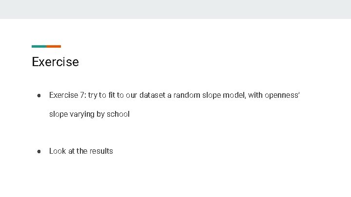
Exercise ● Exercise 7: try to fit to our dataset a random slope model, with openness’ slope varying by school ● Look at the results

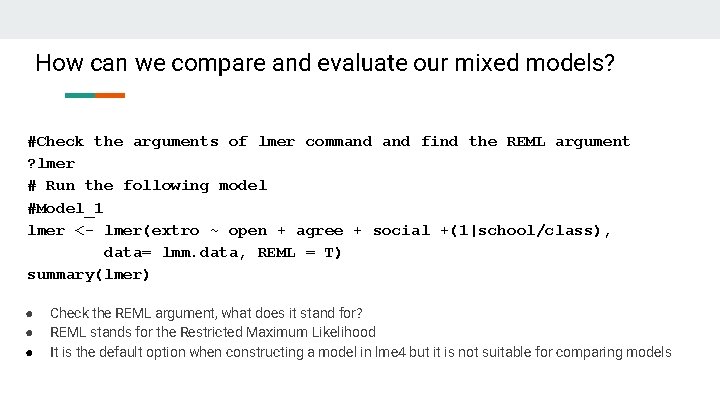
How can we compare and evaluate our mixed models? #Check the arguments of lmer command find the REML argument ? lmer # Run the following model #Model_1 lmer <- lmer(extro ~ open + agree + social +(1|school/class), data= lmm. data, REML = T) summary(lmer) ● ● ● Check the REML argument, what does it stand for? REML stands for the Restricted Maximum Likelihood It is the default option when constructing a model in lme 4 but it is not suitable for comparing models

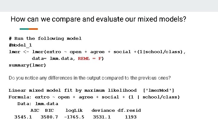
How can we compare and evaluate our mixed models? # Run the following model #Model_1 lmer <- lmer(extro ~ open + agree + social +(1|school/class), data= lmm. data, REML = F) summary(lmer) Do you notice any differences in the output compared to the previous ones? Linear mixed model fit by maximum likelihood ['lmer. Mod'] Formula: extro ~ open + agree + social + (1 | school/class) Data: lmm. data AIC BIC log. Lik deviance df. resid 3545. 1 3580. 7 -1765. 5 3531. 1 1193

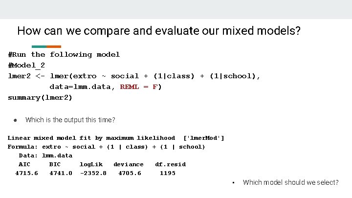
How can we compare and evaluate our mixed models? #Run the following model #Model_2 lmer 2 <- lmer(extro ~ social + (1|class) + (1|school), data=lmm. data, REML = F) summary(lmer 2) ● Which is the output this time? Linear mixed model fit by maximum likelihood ['lmer. Mod'] Formula: extro ~ social + (1 | class) + (1 | school) Data: lmm. data AIC BIC log. Lik deviance df. resid 4715. 6 4741. 0 -2352. 8 4705. 6 1195 • Which model should we select?

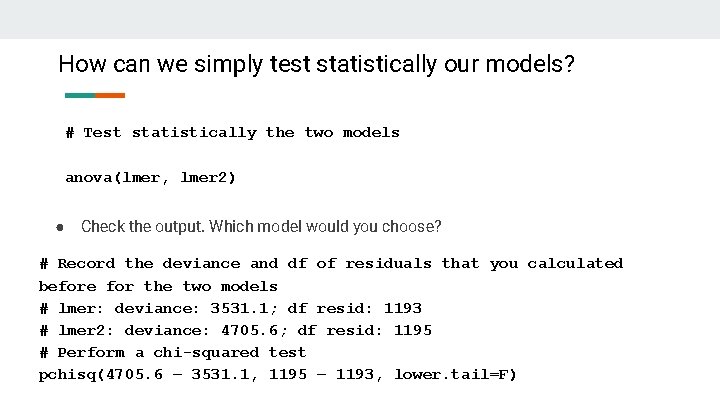
How can we simply test statistically our models? # Test statistically the two models anova(lmer, lmer 2) ● Check the output. Which model would you choose? # Record the deviance and df of residuals that you calculated before for the two models # lmer: deviance: 3531. 1; df resid: 1193 # lmer 2: deviance: 4705. 6; df resid: 1195 # Perform a chi-squared test pchisq(4705. 6 – 3531. 1, 1195 – 1193, lower. tail=F)

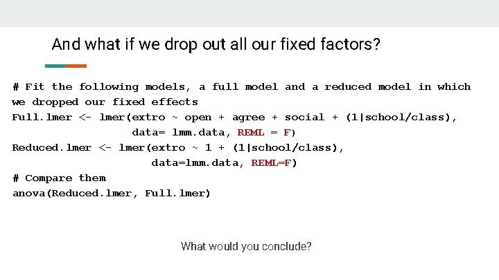
And what if we drop out all our fixed factors? # Fit the following models, a full model and a reduced model in which we dropped our fixed effects Full. lmer <- lmer(extro ~ open + agree + social + (1|school/class), data= lmm. data, REML = F) Reduced. lmer <- lmer(extro ~ 1 + (1|school/class), data=lmm. data, REML=F) # Compare them anova(Reduced. lmer, Full. lmer) What would you conclude?

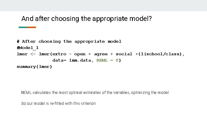
And after choosing the appropriate model? # After choosing the appropriate model #Model_1 lmer <- lmer(extro ~ open + agree + social +(1|school/class), data= lmm. data, REML = T) summary(lmer) REML calculates the most optimal estimates of the variables, optimizing the model So our model is re-fitted with this criterion

Conclusions ● To compare different models with different fixed effects and evaluate the amount of explained information → Maximum Likelihood measures The lower the measures, the better our models fit to the data set ● Depending always on our questions, we construct and select the best fitting models, optimizing them with the REML criterion

THANK YOU FOR YOUR ATTENTION