Fundamentals of Electromagnetics A TwoWeek 8 Day Intensive

Fundamentals of Electromagnetics: A Two-Week, 8 -Day, Intensive Course for Training Faculty in Electrical-, Electronics-, Communication-, and Computer- Related Engineering Departments by Nannapaneni Narayana Rao Edward C. Jordan Professor Emeritus of Electrical and Computer Engineering University of Illinois at Urbana-Champaign, USA Distinguished Amrita Professor of Engineering Amrita Vishwa Vidyapeetham, India Amrita Viswa Vidya Peetham, Coimbatore August 11, 12, 13, 14, 18, 19, 20, and 21, 2008

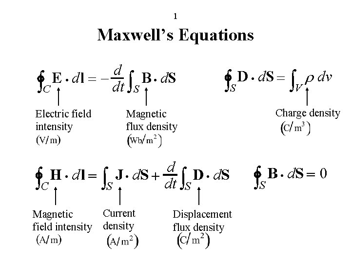
1 Maxwell’s Equations d E × dl = – B × d. S òC dt òS Electric field intensity òS Current density Displacement flux density òV r dv Charge density Magnetic flux density d H × dl = J × d. S + D × d. S òC òS dt òS Magnetic field intensity D × d. S = òS B × d. S = 0

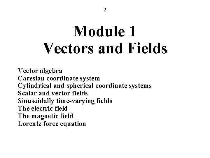
2 Module 1 Vectors and Fields Vector algebra Caresian coordinate system Cylindrical and spherical coordinate systems Scalar and vector fields Sinusoidally time-varying fields The electric field The magnetic field Lorentz force equation

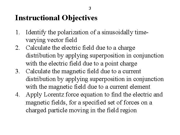
3 Instructional Objectives 1. Identify the polarization of a sinusoidally timevarying vector field 2. Calculate the electric field due to a charge distribution by applying superposition in conjunction with the electric field due to a point charge 3. Calculate the magnetic field due to a current distribution by applying superposition in conjunction with the magnetic field due to a current element 4. Apply Lorentz force equation to find the electric and magnetic fields, for a specified set of forces on a charged particle moving in the field region

4 Vector Algebra (FEME, Sec. 1. 1; EEE 6 E, Sec. 1. 1) In this series of Power. Point presentations, FEME refers to “Fundamentals of Electromagnetics for Electrical and Computer Engineering, ” U. S. and International Editions (2009), or “Fundamentals of Electromagnetics for Engineering, ” Indian Edition (2009), and EEE 6 E refers to “Elements of Engineering Electromagnetics, 6 th Edition, ” U. S. and International Editions (2004) or Indian Edition (2006).

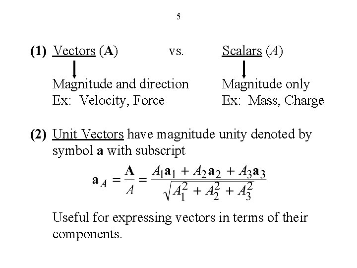
5 (1) Vectors (A) vs. Magnitude and direction Ex: Velocity, Force Scalars (A) Magnitude only Ex: Mass, Charge (2) Unit Vectors have magnitude unity denoted by symbol a with subscript Useful for expressing vectors in terms of their components.

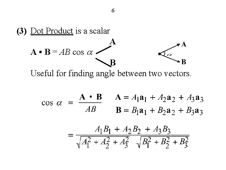
6 (3) Dot Product is a scalar A A • B = AB cos a B Useful for finding angle between two vectors.

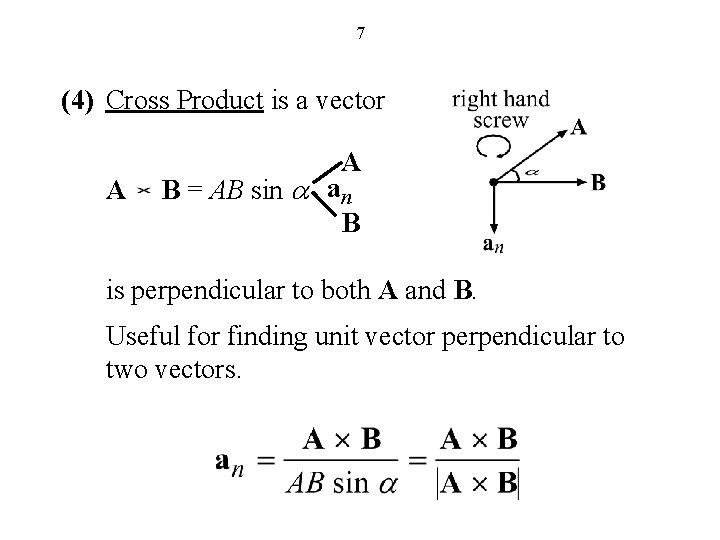
7 (4) Cross Product is a vector A A B = AB sin a an B is perpendicular to both A and B. Useful for finding unit vector perpendicular to two vectors.

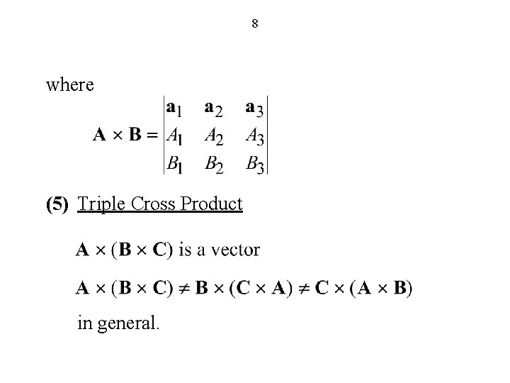
8 where (5) Triple Cross Product in general.

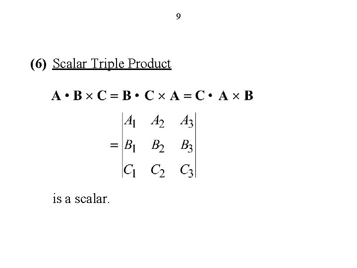
9 (6) Scalar Triple Product is a scalar.

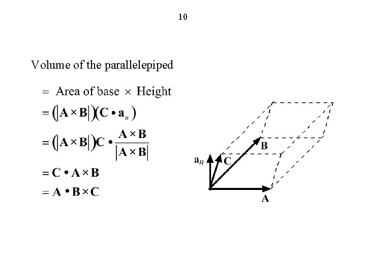
10 Volume of the parallelepiped

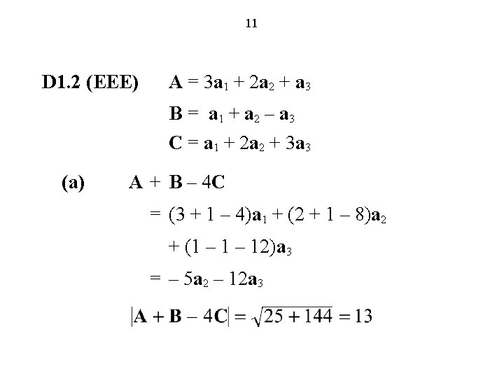
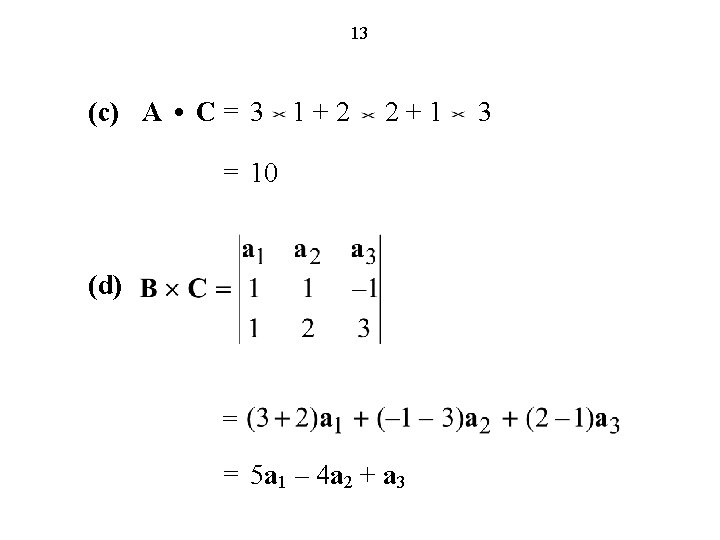
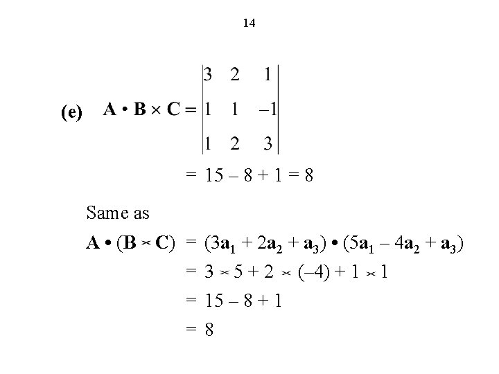
11 D 1. 2 (EEE) A = 3 a 1 + 2 a 2 + a 3 B = a 1 + a 2 – a 3 C = a 1 + 2 a 2 + 3 a 3 (a) A + B – 4 C = (3 + 1 – 4)a 1 + (2 + 1 – 8)a 2 + (1 – 12)a 3 = – 5 a 2 – 12 a 3

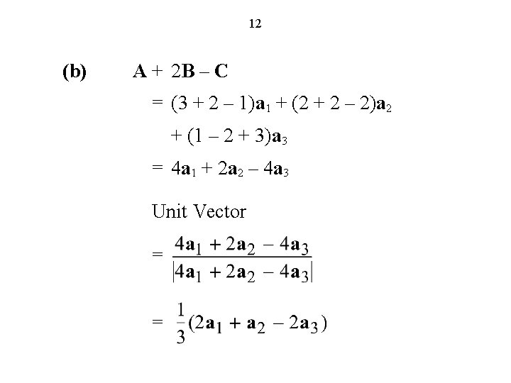
12 (b) A + 2 B – C = (3 + 2 – 1)a 1 + (2 + 2 – 2)a 2 + (1 – 2 + 3)a 3 = 4 a 1 + 2 a 2 – 4 a 3 Unit Vector = =

13 (c) A • C = 3 1 + 2 2 + 1 3 = 10 (d) = = 5 a 1 – 4 a 2 + a 3

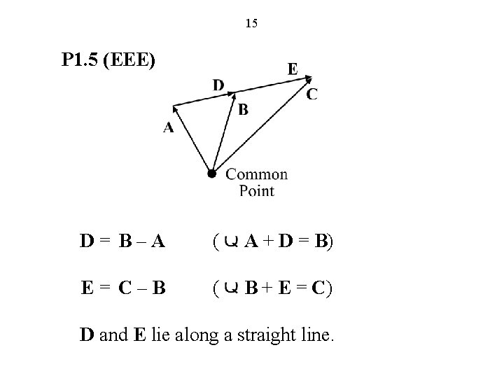
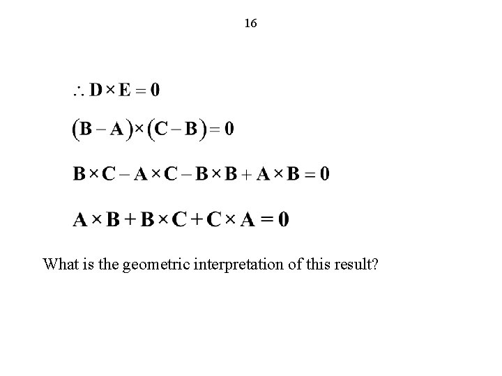
15 P 1. 5 (EEE) D = B – A ( A + D = B) E = C – B ( B + E = C) D and E lie along a straight line.

16 What is the geometric interpretation of this result?

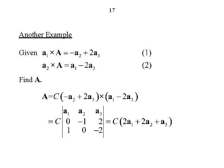
17 Another Example Given Find A.

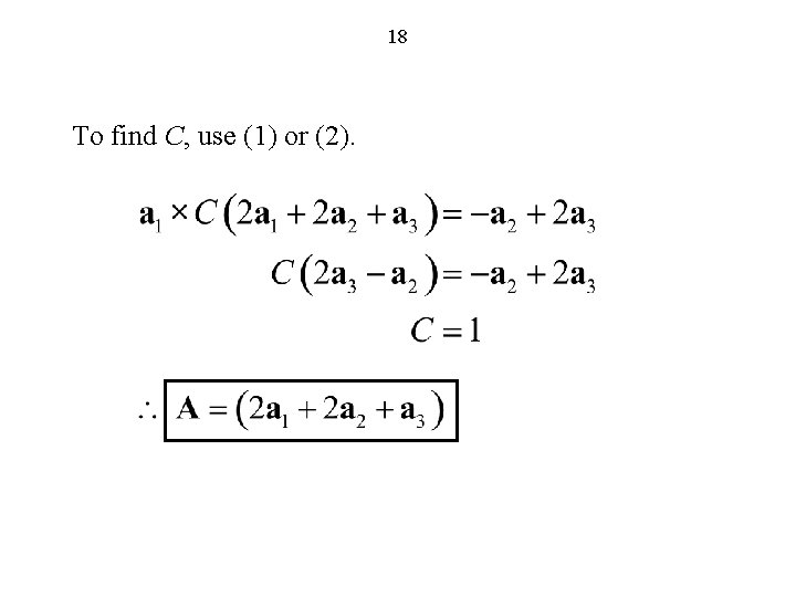
18 To find C, use (1) or (2).

19 Cartesian Coordinate System (FEME, Sec. 1. 2; EEE 6 E, Sec. 1. 2)

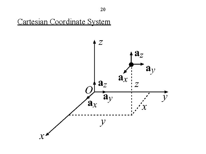
20 Cartesian Coordinate System

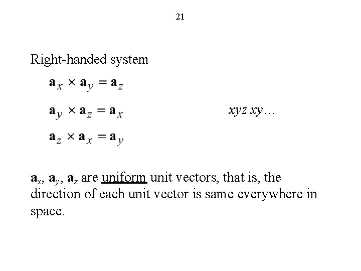
21 Right-handed system xyz xy… ax, ay, az are uniform unit vectors, that is, the direction of each unit vector is same everywhere in space.

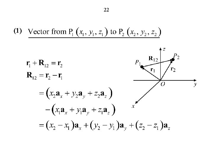
22 (1)

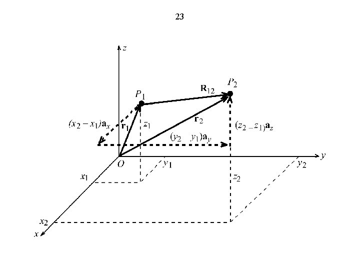
23

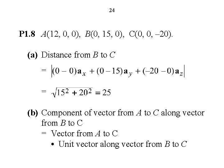
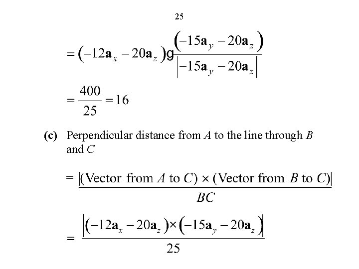
24 P 1. 8 A(12, 0, 0), B(0, 15, 0), C(0, 0, – 20). (a) Distance from B to C = = (b) Component of vector from A to C along vector from B to C = Vector from A to C • Unit vector along vector from B to C

25 (c) Perpendicular distance from A to the line through B and C =

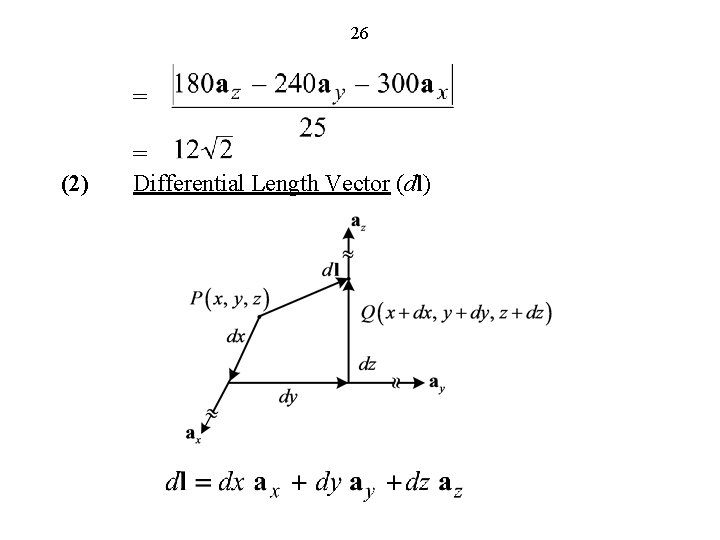
26 = (2) = Differential Length Vector (dl)

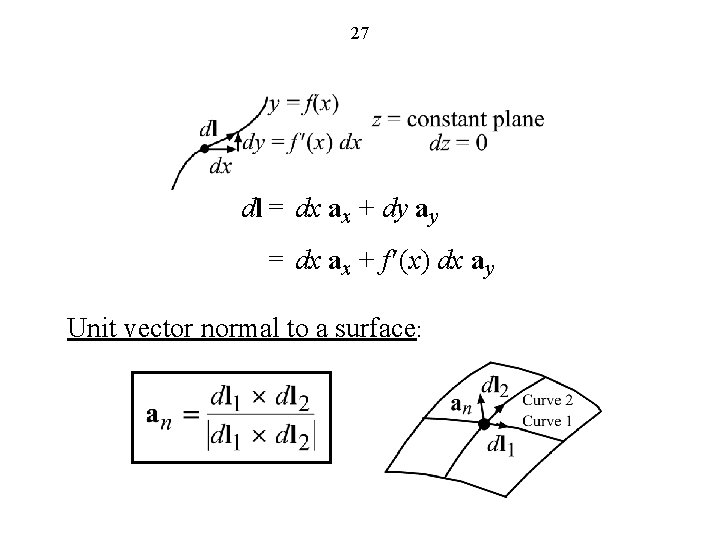
27 dl = dx ax + dy ay = dx ax + f ¢(x) dx ay Unit vector normal to a surface:

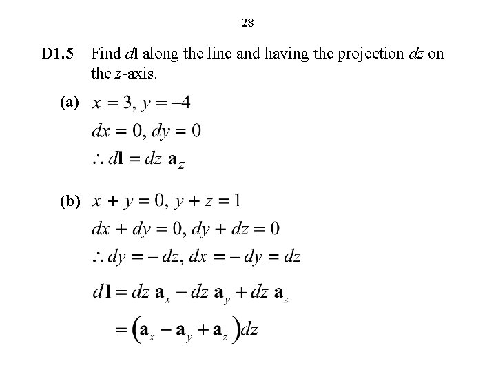
28 D 1. 5 (a) (b) Find dl along the line and having the projection dz on the z-axis.

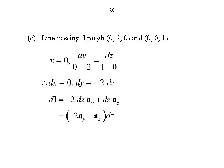
29 (c) Line passing through (0, 2, 0) and (0, 0, 1).

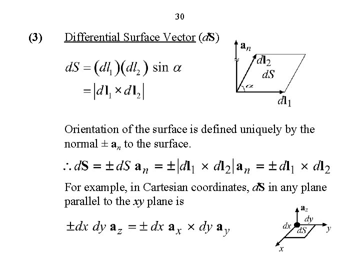
30 (3) Differential Surface Vector (d. S) Orientation of the surface is defined uniquely by the normal ± an to the surface. For example, in Cartesian coordinates, d. S in any plane parallel to the xy plane is

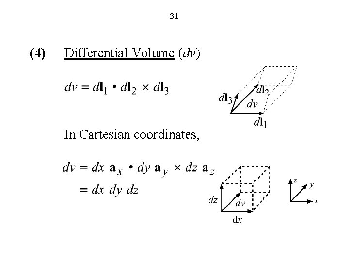
31 (4) Differential Volume (dv) In Cartesian coordinates,

32 Cylindrical and Spherical Coordinate Systems (FEME, Appendix A; EEE 6 E, Sec. 1. 3)

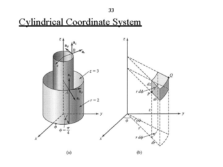
33 Cylindrical Coordinate System

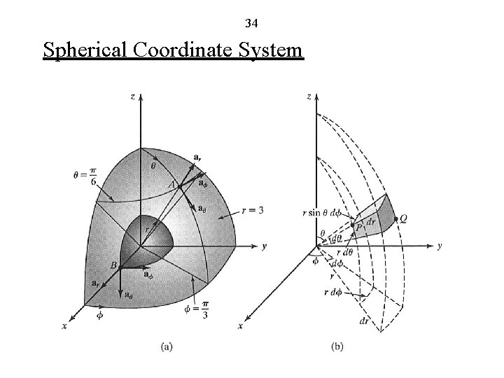
34 Spherical Coordinate System

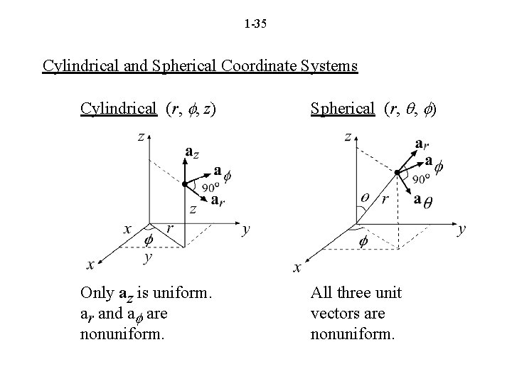
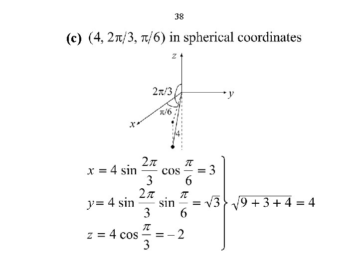
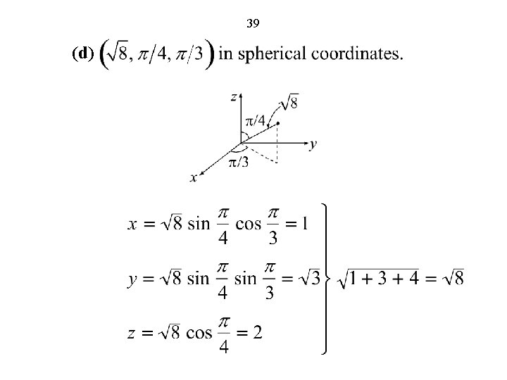
1 -35 Cylindrical and Spherical Coordinate Systems Cylindrical (r, f, z) Spherical (r, q, f) Only az is uniform. ar and af are nonuniform. All three unit vectors are nonuniform.

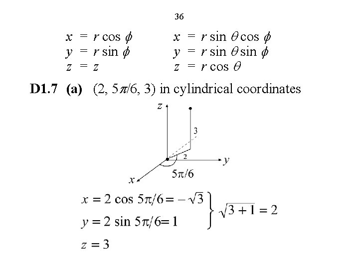
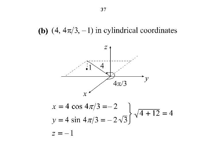
36 x = r cos f y = r sin f z =z x = r sin q cos f y = r sin q sin f z = r cos q D 1. 7 (a) (2, 5 p/6, 3) in cylindrical coordinates

37 (b)

38 (c)

39 (d)

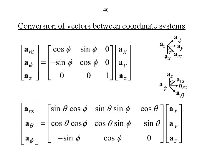
40 Conversion of vectors between coordinate systems

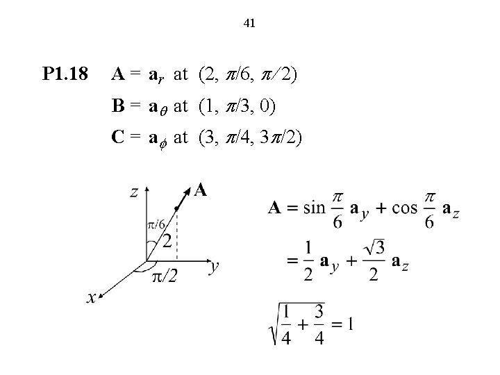
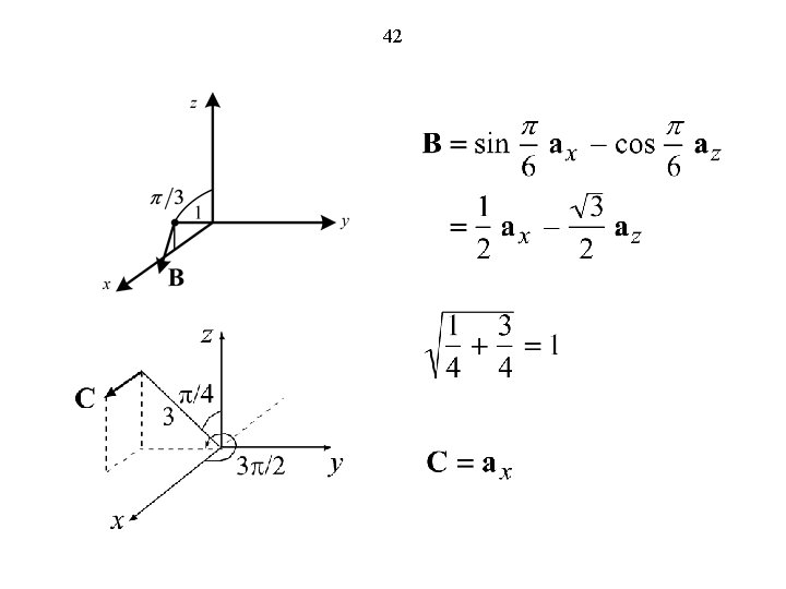
41 P 1. 18 A = ar at (2, p/6, p/ 2) B = aq at (1, p/3, 0) C = af at (3, p/4, 3 p/2)

42

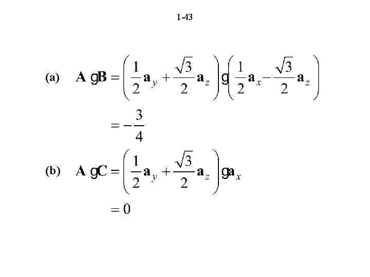
1 -43 (a) (b)

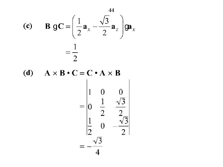
44 (c) (d)

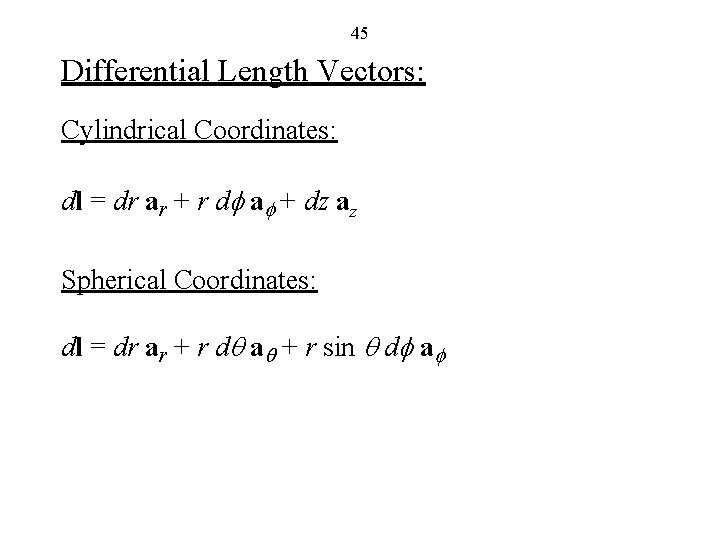
45 Differential Length Vectors: Cylindrical Coordinates: dl = dr ar + r df af + dz az Spherical Coordinates: dl = dr ar + r dq aq + r sin q df af

46 Scalar and Vector Fields (FEME, Sec. 1. 3; EEE 6 E, Sec. 1. 4)

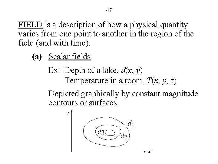
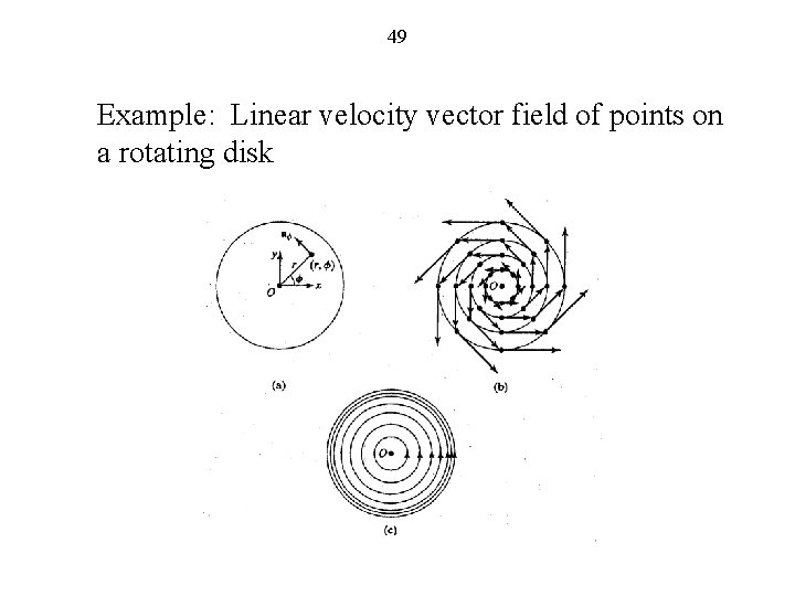
47 FIELD is a description of how a physical quantity varies from one point to another in the region of the field (and with time). (a) Scalar fields Ex: Depth of a lake, d(x, y) Temperature in a room, T(x, y, z) Depicted graphically by constant magnitude contours or surfaces.

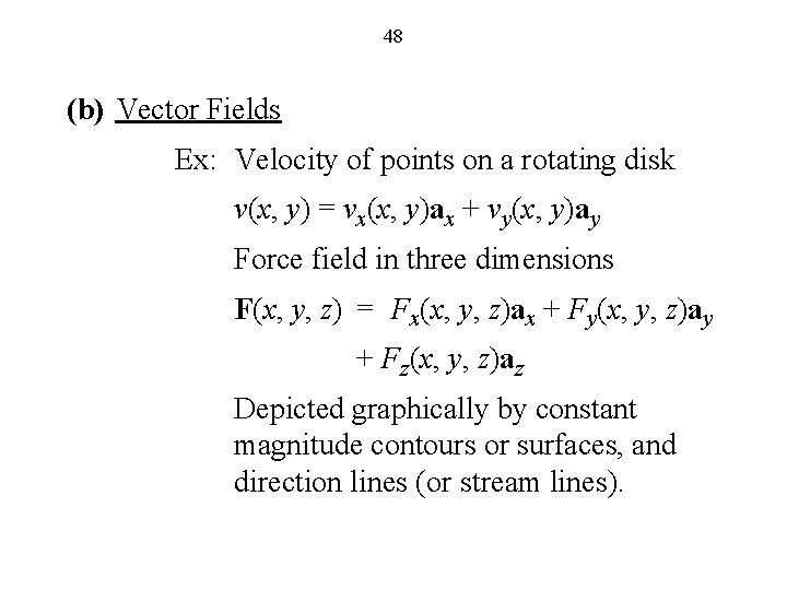
48 (b) Vector Fields Ex: Velocity of points on a rotating disk v(x, y) = vx(x, y)ax + vy(x, y)ay Force field in three dimensions F(x, y, z) = Fx(x, y, z)ax + Fy(x, y, z)ay + Fz(x, y, z)az Depicted graphically by constant magnitude contours or surfaces, and direction lines (or stream lines).

49 Example: Linear velocity vector field of points on a rotating disk

50 (c) Static Fields not varying with time. (d) Dynamic Fields varying with time. Ex: Temperature in a room, T(x, y, z; t)

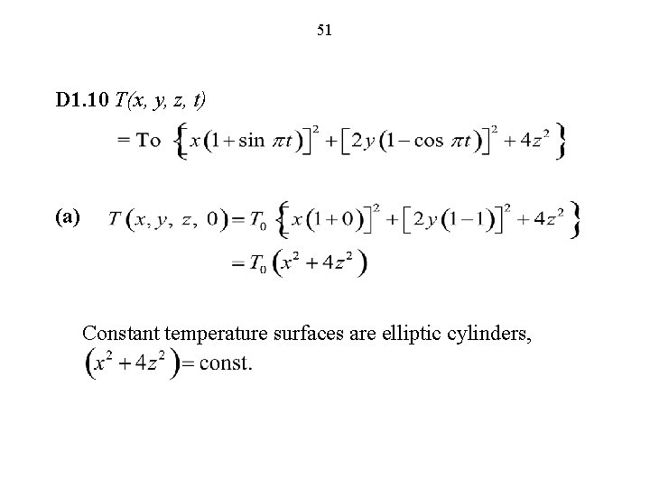
51 D 1. 10 T(x, y, z, t) (a) Constant temperature surfaces are elliptic cylinders,

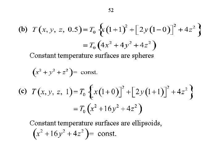
52 (b) Constant temperature surfaces are spheres (c) Constant temperature surfaces are ellipsoids,

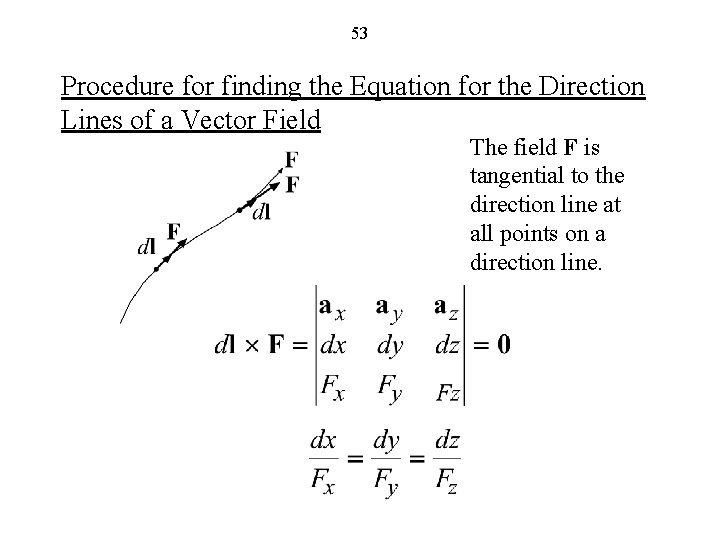
53 Procedure for finding the Equation for the Direction Lines of a Vector Field The field F is tangential to the direction line at all points on a direction line.

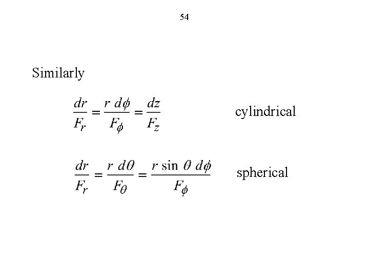
54 Similarly cylindrical spherical

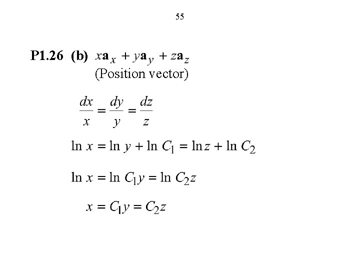
55 P 1. 26 (b) (Position vector)

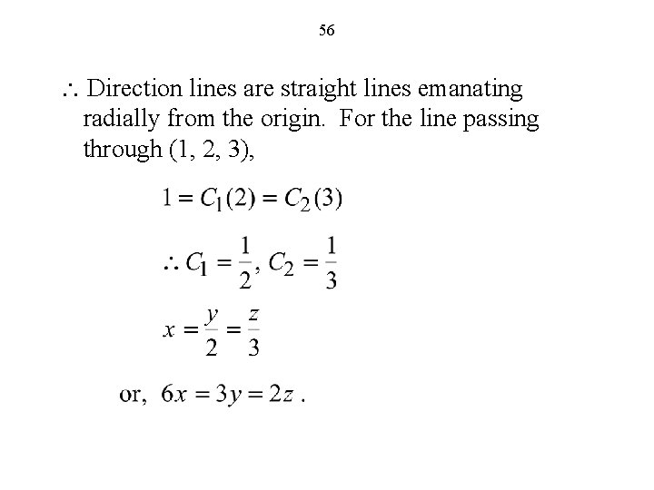
56 Direction lines are straight lines emanating radially from the origin. For the line passing through (1, 2, 3),

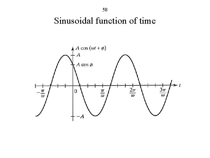
57 Sinusoidally Time-Varying Fields (FEME, Sec. 1. 4; EEE 6 E, Sec. 3. 6)

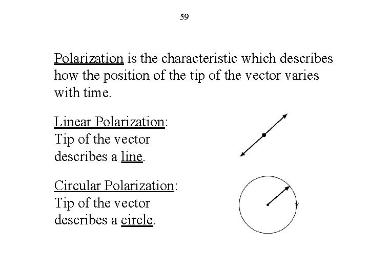
58 Sinusoidal function of time

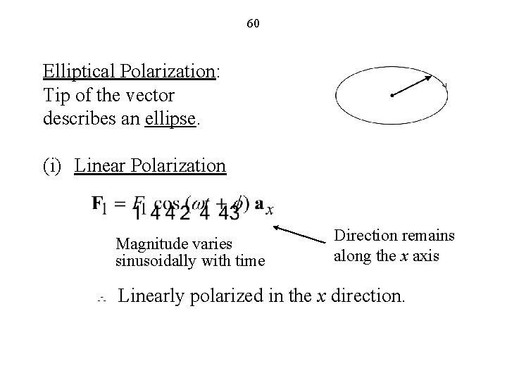
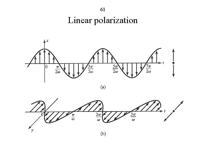
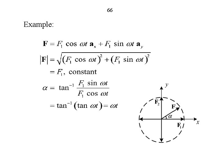
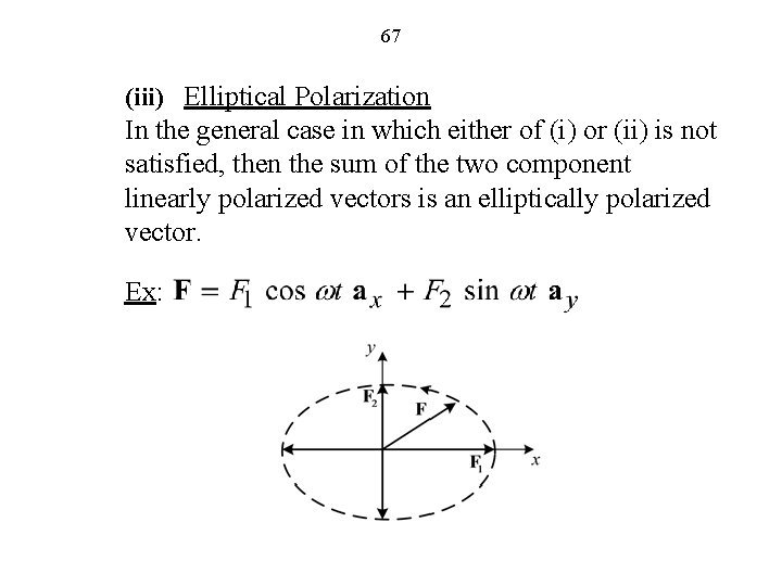
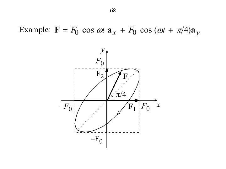
59 Polarization is the characteristic which describes how the position of the tip of the vector varies with time. Linear Polarization: Tip of the vector describes a line. Circular Polarization: Tip of the vector describes a circle.

60 Elliptical Polarization: Tip of the vector describes an ellipse. (i) Linear Polarization Magnitude varies sinusoidally with time Direction remains along the x axis Linearly polarized in the x direction.

61 Linear polarization

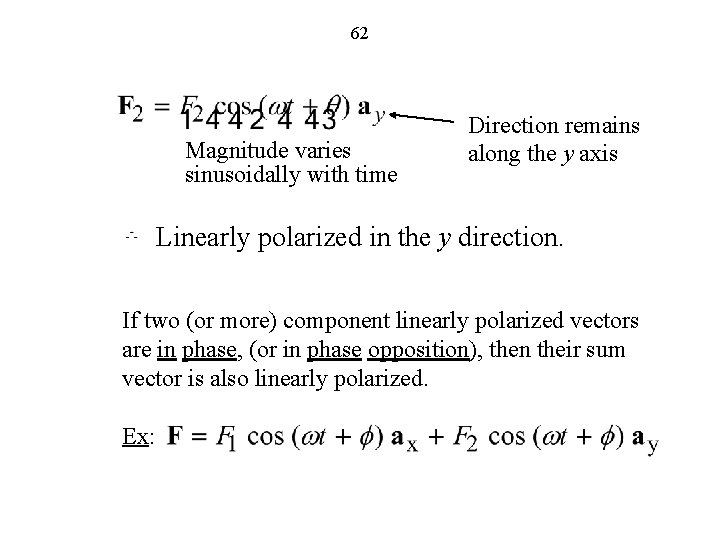
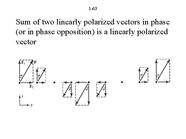
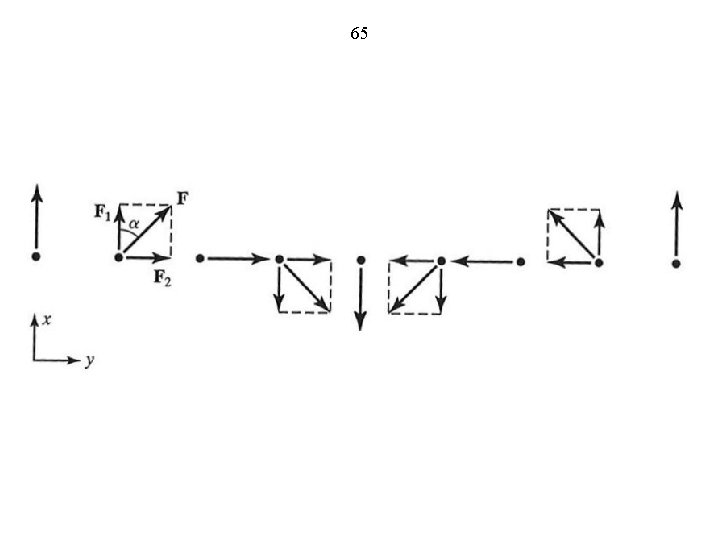
62 Magnitude varies sinusoidally with time Direction remains along the y axis Linearly polarized in the y direction. If two (or more) component linearly polarized vectors are in phase, (or in phase opposition), then their sum vector is also linearly polarized. Ex:

1 -63 Sum of two linearly polarized vectors in phase (or in phase opposition) is a linearly polarized vector

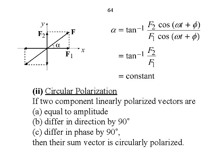
64 (ii) Circular Polarization If two component linearly polarized vectors are (a) equal to amplitude (b) differ in direction by 90˚ (c) differ in phase by 90˚, then their sum vector is circularly polarized.

65

66 Example:

67 (iii) Elliptical Polarization In the general case in which either of (i) or (ii) is not satisfied, then the sum of the two component linearly polarized vectors is an elliptically polarized vector. Ex:

68 Example:

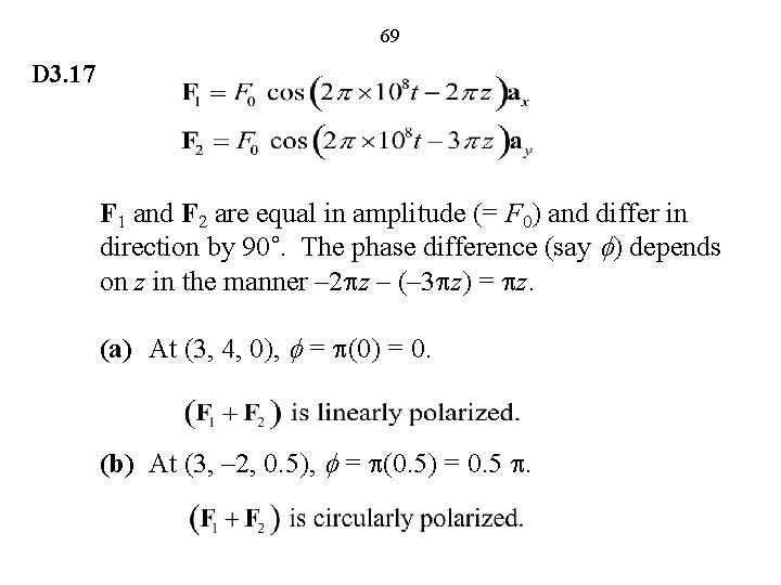
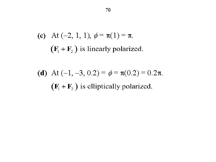
69 D 3. 17 F 1 and F 2 are equal in amplitude (= F 0) and differ in direction by 90˚. The phase difference (say f) depends on z in the manner – 2 pz – (– 3 pz) = pz. (a) At (3, 4, 0), f = p(0) = 0. (b) At (3, – 2, 0. 5), f = p(0. 5) = 0. 5 p.

71 The Electric Field (FEME, Sec. 1. 5; EEE 6 E, Sec. 1. 5)

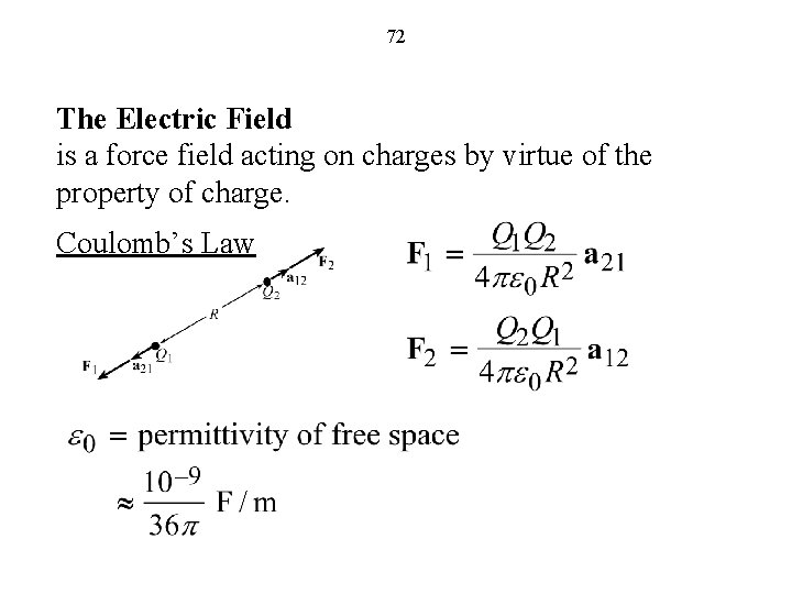
72 The Electric Field is a force field acting on charges by virtue of the property of charge. Coulomb’s Law

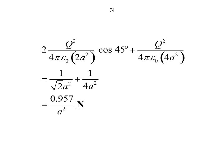
73 D 1. 13(b) Q 2/4 pe 0(2 a 2) Q 2/4 pe 0(4 a 2) Q 2/4 pe 0(2 a 2) From the construction, it is evident that the resultant force is directed away from the center of the square. The magnitude of this resultant force is given by

74

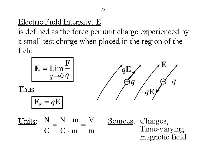
75 Electric Field Intensity, E is defined as the force per unit charge experienced by a small test charge when placed in the region of the field. Thus Units: Sources: Charges; Time-varying magnetic field

76 Electric Field of a Point Charge (Coulomb’s Law)

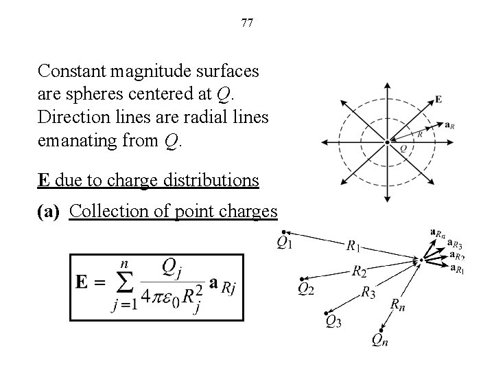
77 Constant magnitude surfaces are spheres centered at Q. Direction lines are radial lines emanating from Q. E due to charge distributions (a) Collection of point charges

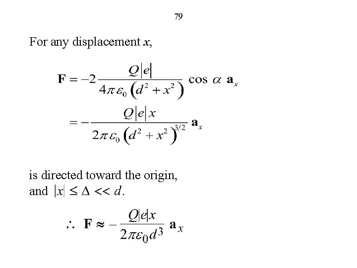
78 Ex. a Electron (charge e and mass m) is displaced from the origin by D (<< d) in the +x-direction and released from rest at t = 0. We wish to obtain differential equation for the motion of the electron and its solution.

79 For any displacement x, is directed toward the origin, and

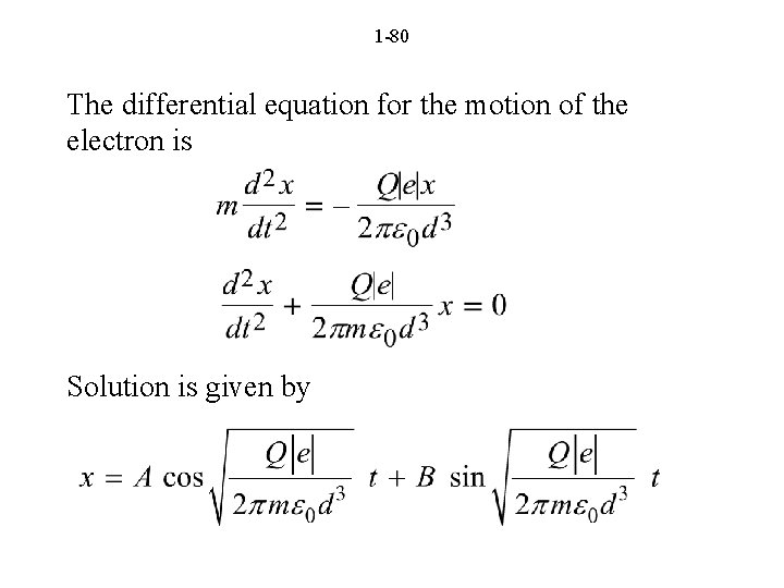
1 -80 The differential equation for the motion of the electron is Solution is given by

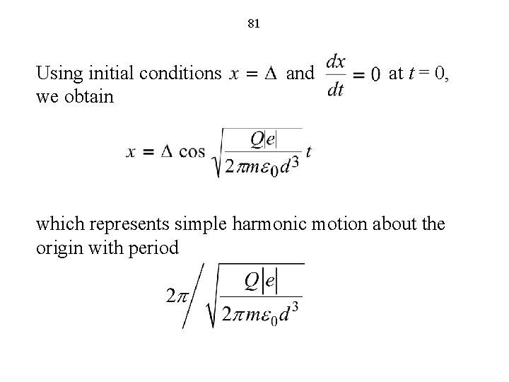
81 Using initial conditions and at t = 0, we obtain which represents simple harmonic motion about the origin with period

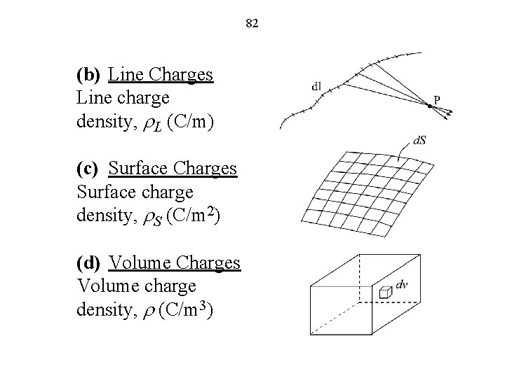
82 (b) Line Charges Line charge density, r. L (C/m) (c) Surface Charges Surface charge density, r. S (C/m 2) (d) Volume Charges Volume charge density, r (C/m 3)

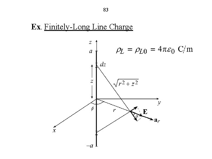
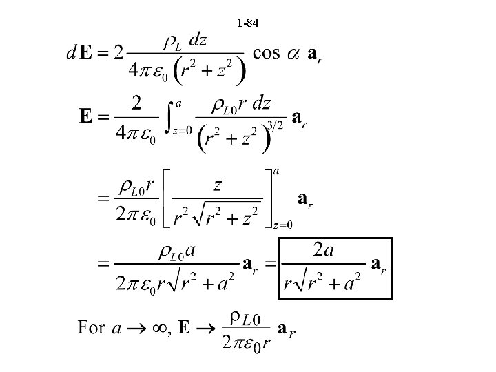
83 Ex. Finitely-Long Line Charge f a

1 -84

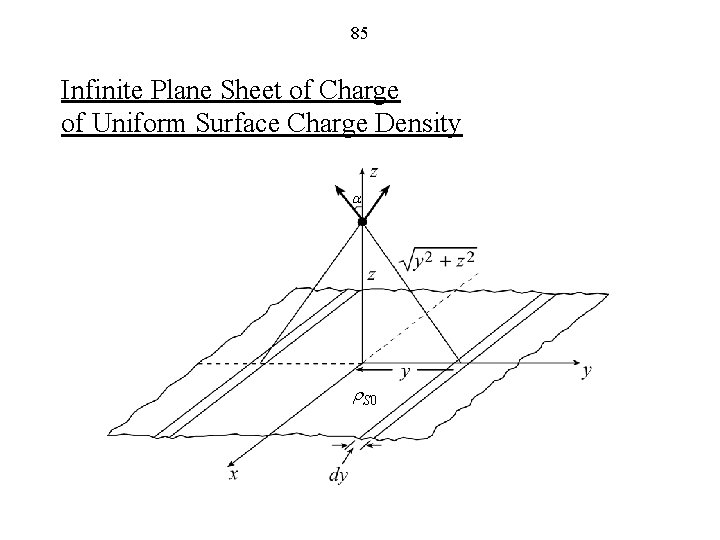
85 Infinite Plane Sheet of Charge of Uniform Surface Charge Density a r. S 0

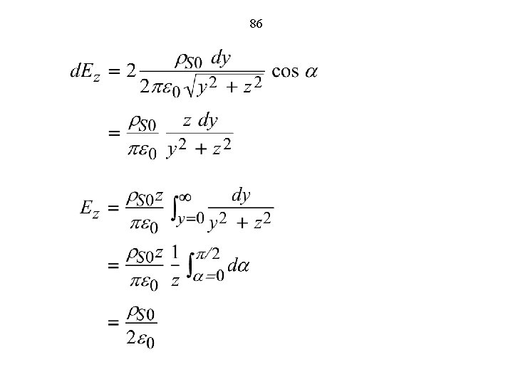
86

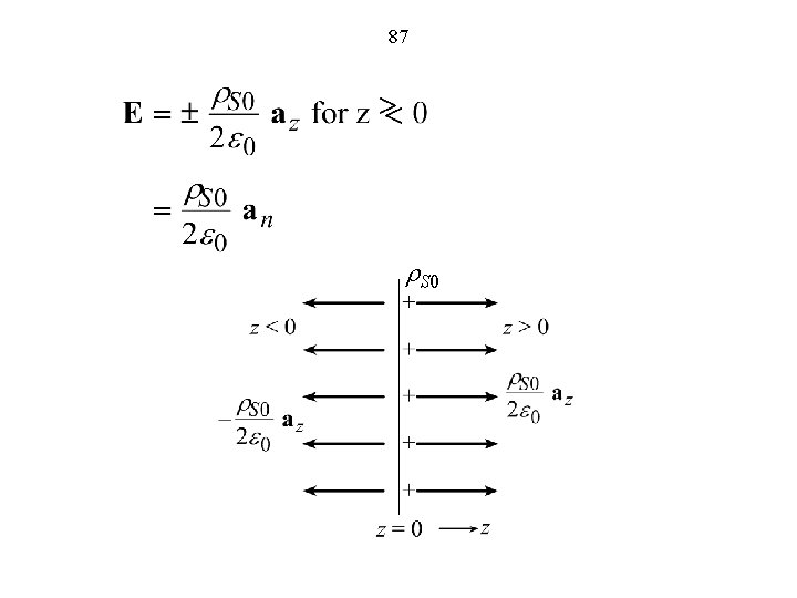
87 r. S 0

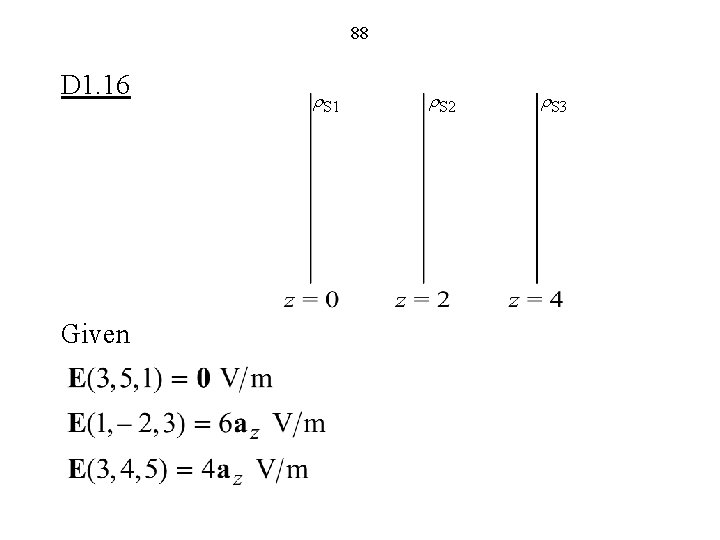
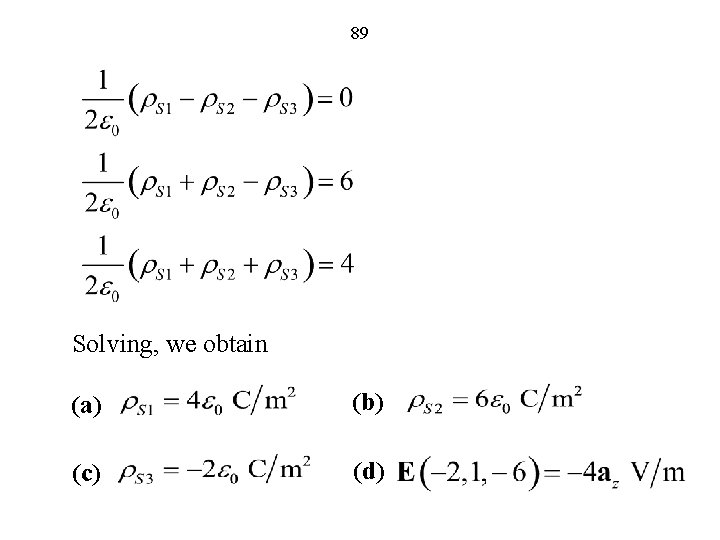
88 D 1. 16 Given r. S 1 r. S 2 r. S 3

89 Solving, we obtain (a) (b) (c) (d)

90 The Magnetic Field (FEME, Sec. 1. 6; EEE 6 E, Sec. 1. 6)

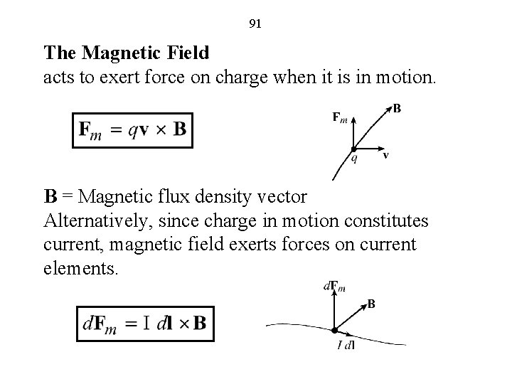
91 The Magnetic Field acts to exert force on charge when it is in motion. B = Magnetic flux density vector Alternatively, since charge in motion constitutes current, magnetic field exerts forces on current elements.

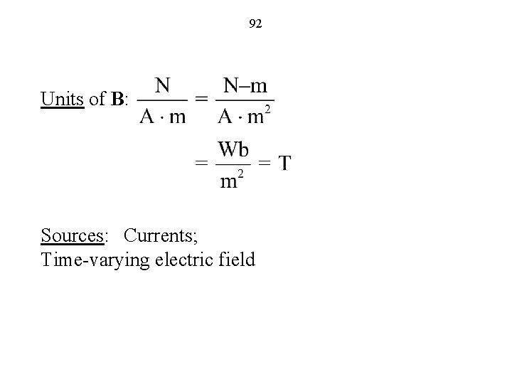
92 Units of B: Sources: Currents; Time-varying electric field

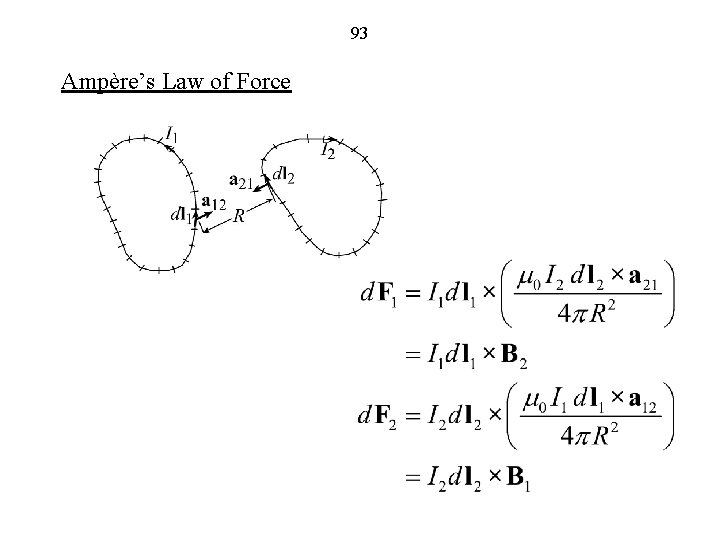
93 Ampère’s Law of Force

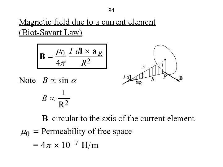
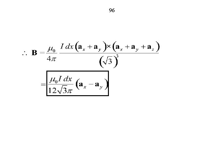
94 Magnetic field due to a current element (Biot-Savart Law) a B circular to the axis of the current element

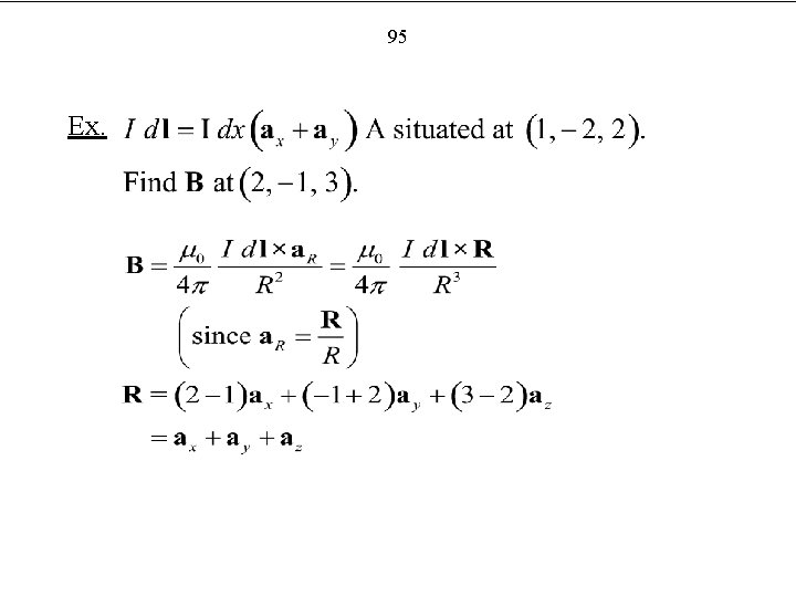
95 Ex.

96

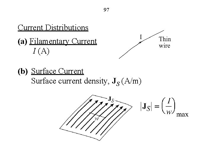
97 Current Distributions (a) Filamentary Current I (A) (b) Surface Current Surface current density, JS (A/m)

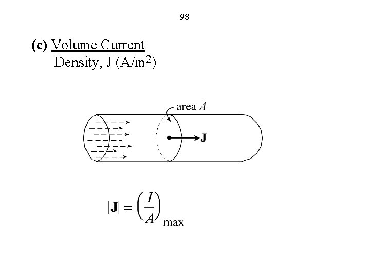
98 (c) Volume Current Density, J (A/m 2)

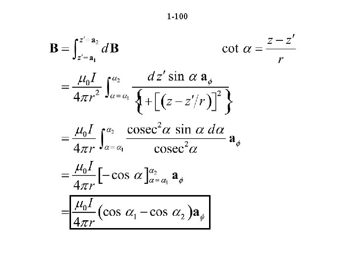
99 P 1. 44 a 2 a a 1 P(r, f, z)

1 -100

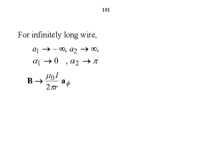
101 For infinitely long wire,

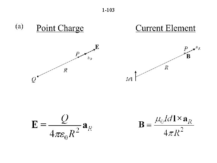
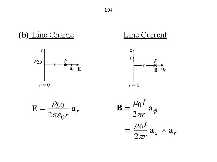
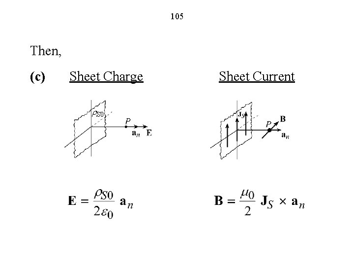
102 Magnetic Field Due to an Infinite Plane Sheet of Uniform Surface Current Density This can be found by dividing the sheet into infinitely long strips parallel to the current density and using superposition, as in the case of finding the electric field due to an infinite plane sheet of uniform surface charge density. Instead of going through this procedure, let us use analogy. To do this, we first note the following:

1 -103

104 (b) Line Charge r. L 0 Line Current

105 Then, (c) Sheet Charge r. S 0 Sheet Current

106 Lorentz Force Equation (FEME, Sec. 1. 6; EEE 6 E, Sec. 1. 7)

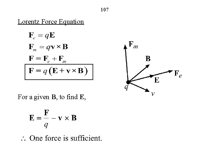
107 Lorentz Force Equation For a given B, to find E,

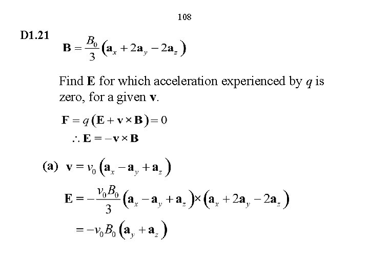
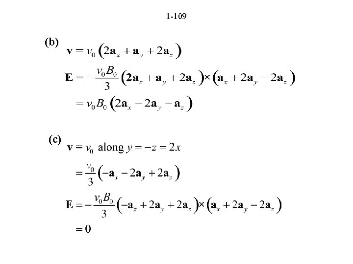
108 D 1. 21 Find E for which acceleration experienced by q is zero, for a given v. (a)

1 -109 (b) (c)

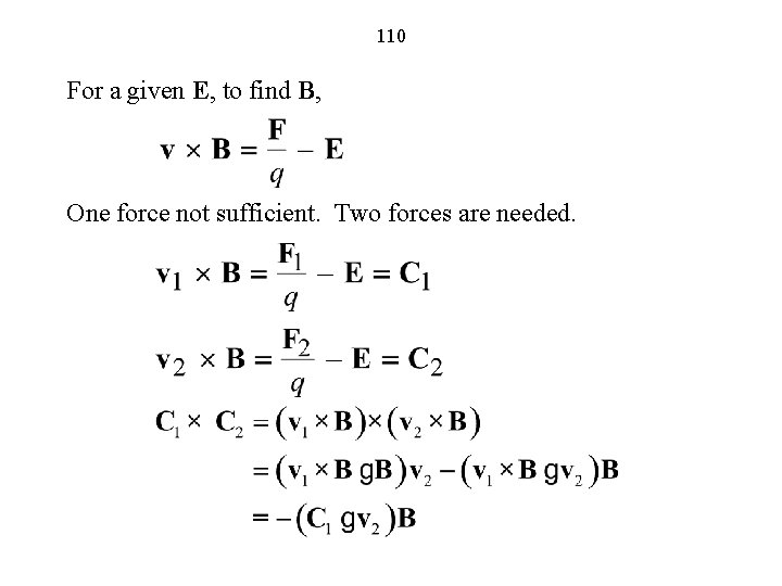
110 For a given E, to find B, One force not sufficient. Two forces are needed.

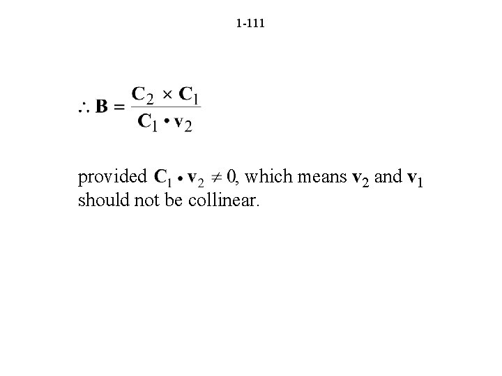
1 -111 provided , which means v 2 and v 1 should not be collinear.

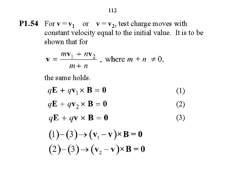
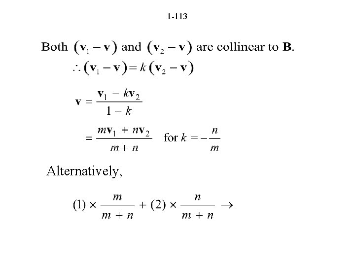
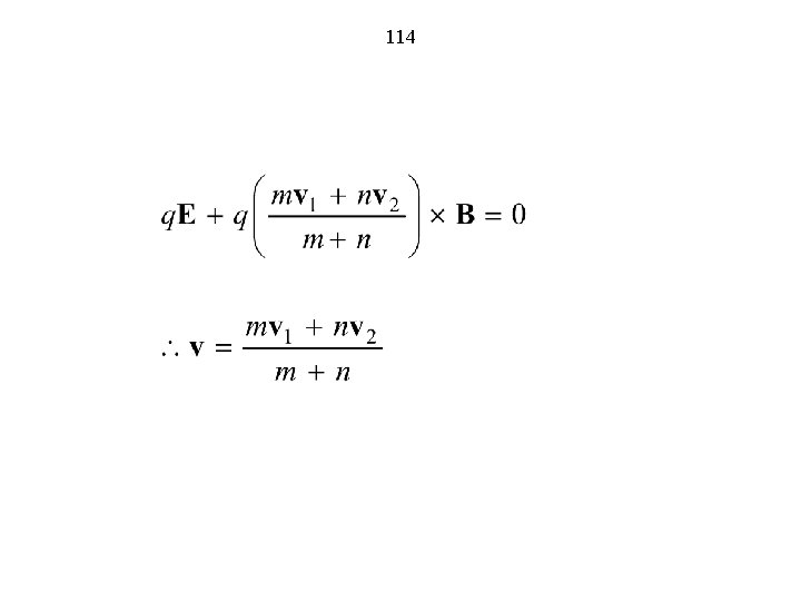
112 P 1. 54 For v = v 1 or v = v 2, test charge moves with constant velocity equal to the initial value. It is to be shown that for the same holds. (1) (2) (3)

1 -113 Alternatively,

114

The End