Forecasting To Accompany Russell and Taylor Operations Management

Forecasting To Accompany Russell and Taylor, Operations Management, 4 th Edition, 2003 Prentice-Hall, Inc. All rights reserved.

Forecasting ü Predicting future events ü Usually demand behavior over a time frame

Forecast: • A statement about the future value of a variable of interest such as demand. • Forecasts affect decisions and activities throughout an organization – Accounting, finance – Human resources – Marketing – MIS – Operations – Product / service design

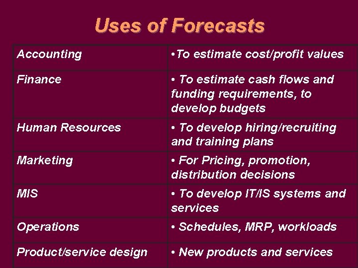
Uses of Forecasts Accounting • To estimate cost/profit values Finance • To estimate cash flows and funding requirements, to develop budgets Human Resources • To develop hiring/recruiting and training plans Marketing • For Pricing, promotion, distribution decisions MIS • To develop IT/IS systems and services Operations • Schedules, MRP, workloads Product/service design • New products and services

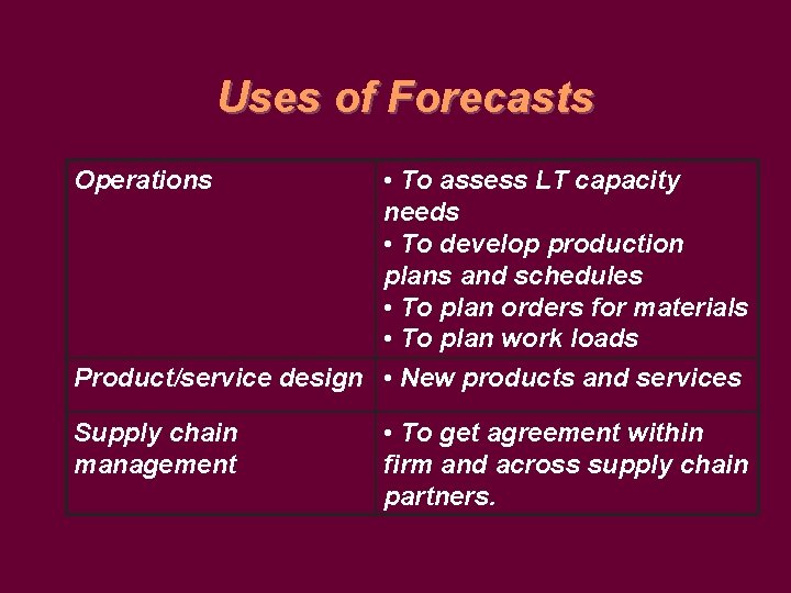
Uses of Forecasts • To assess LT capacity needs • To develop production plans and schedules • To plan orders for materials • To plan work loads Product/service design • New products and services Operations Supply chain management • To get agreement within firm and across supply chain partners.

Uses of Forecasts: Summary Ø To help managers plan the system Ø To help managers plan the use of the system.

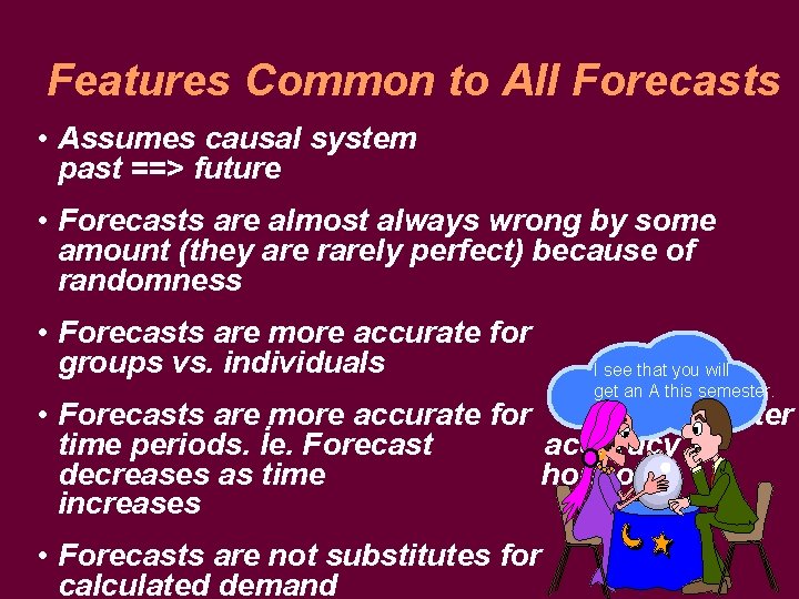
Features Common to All Forecasts • Assumes causal system past ==> future • Forecasts are almost always wrong by some amount (they are rarely perfect) because of randomness • Forecasts are more accurate for groups vs. individuals I see that you will get an A this semester. • Forecasts are more accurate for shorter time periods. İe. Forecast accuracy decreases as time horizon increases • Forecasts are not substitutes for calculated demand

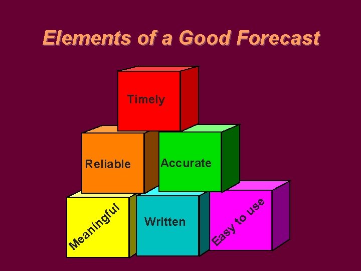
Elements of a Good Forecast Timely Reliable M e ul f ng i an Accurate Written y s Ea to e s u

Time Frame in Forecasting ü Short-range to medium-range ü Daily, weekly monthly forecasts of sales data ü Up to 2 years into the future ü Long-range ü Strategic planning of goals, products, markets ü Planning beyond 2 years into the future

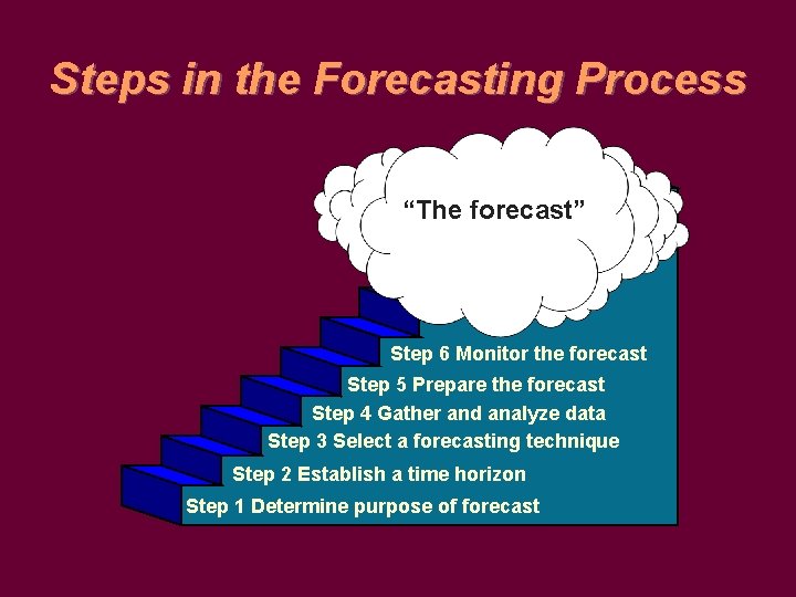
Steps in the Forecasting Process “The forecast” Step 6 Monitor the forecast Step 5 Prepare the forecast Step 4 Gather and analyze data Step 3 Select a forecasting technique Step 2 Establish a time horizon Step 1 Determine purpose of forecast

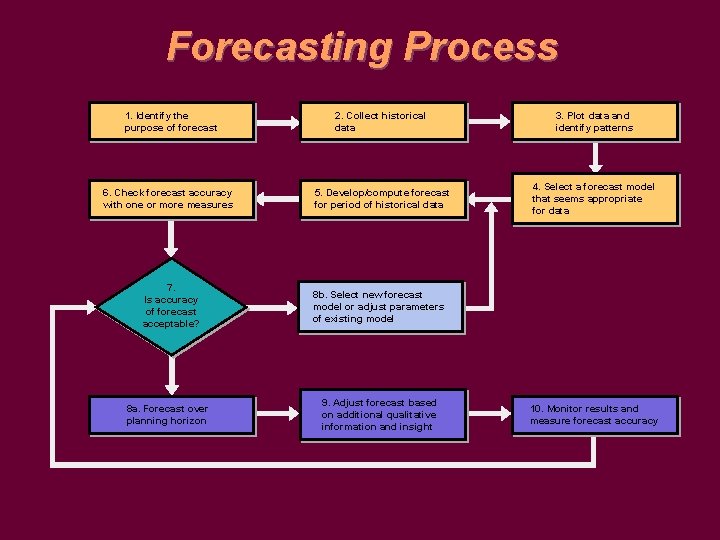
Forecasting Process 1. Identify the purpose of forecast 2. Collect historical data 3. Plot data and identify patterns 6. Check forecast accuracy with one or more measures 5. Develop/compute forecast for period of historical data 4. Select a forecast model that seems appropriate for data 7. Is accuracy of forecast acceptable? 8 a. Forecast over planning horizon 8 b. Select new forecast model or adjust parameters of existing model 9. Adjust forecast based on additional qualitative information and insight 10. Monitor results and measure forecast accuracy

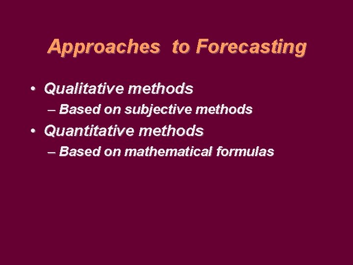
Approaches to Forecasting • Qualitative methods – Based on subjective methods • Quantitative methods – Based on mathematical formulas

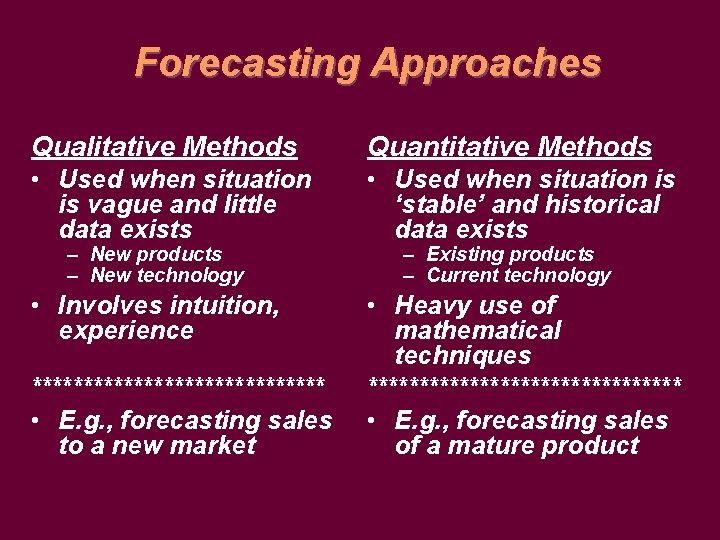
Forecasting Approaches Qualitative Methods Quantitative Methods • Used when situation is vague and little data exists • Used when situation is ‘stable’ and historical data exists • Involves intuition, experience • Heavy use of mathematical techniques **************** • E. g. , forecasting sales of a mature product – New products – New technology *************** • E. g. , forecasting sales to a new market – Existing products – Current technology

“Q 2” Forecasting Quantitative, then qualitative factors to “filter” the answer

Approaches to Forecasting • Judgmental (Qualitative)- uses subjective inputs • Time series - uses historical data assuming the future will be like the past • Associative models - uses explanatory variables to predict the future

Qualitative (Judgmental)Forecasting • Executive opinions • Sales force opinions • Consumer surveys • Outside opinion • Delphi method – Opinions of managers and staff – Achieves a consensus forecast

Time Series A time series is a time-ordered sequence of observations taken at regular intervals (eg. Hourly, daily, weekly, monthly, quarterly, annually)

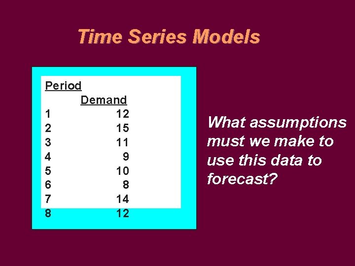
Time Series Models Period Demand 1 12 2 15 3 11 4 9 5 10 6 8 7 14 8 12 What assumptions must we make to use this data to forecast?

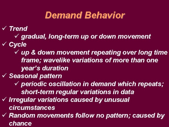
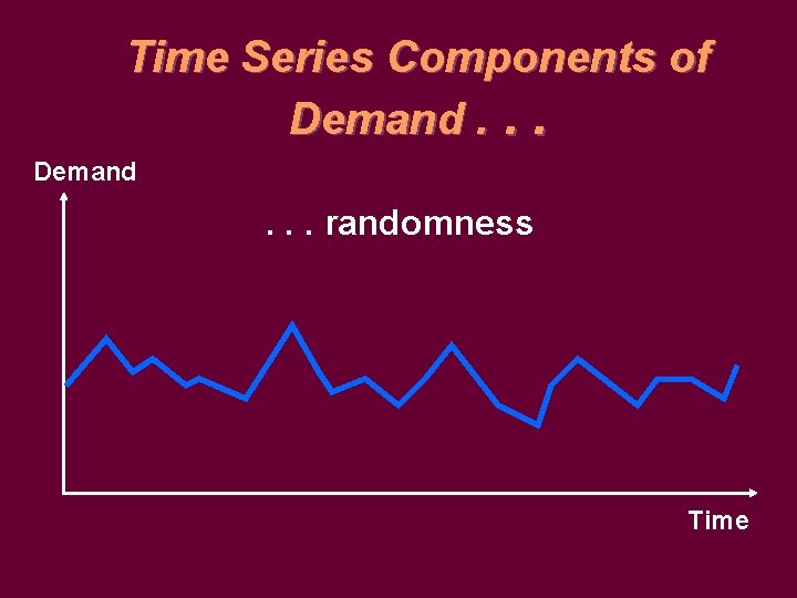
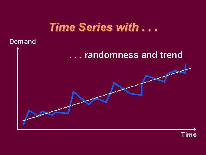
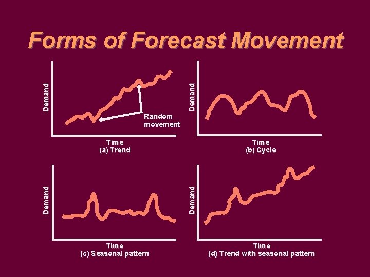
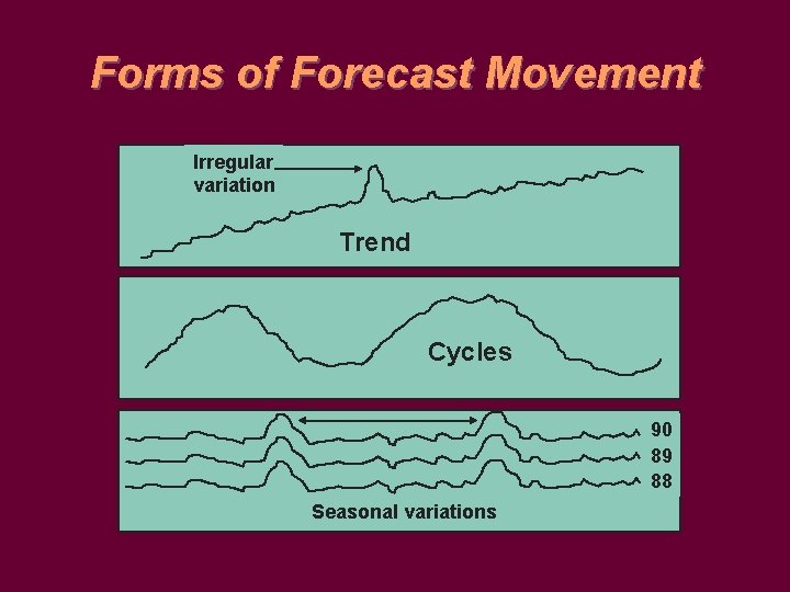
Demand Behavior ü Trend ü gradual, long-term up or down movement ü Cycle ü up & down movement repeating over long time frame; wavelike variations of more than one year’s duration ü Seasonal pattern ü periodic oscillation in demand which repeats; short-term regular variations in data ü Irregular variations caused by unusual circumstances ü Random movements follow no pattern; caused by chance

Time Series Components of Demand. . . Demand . . . randomness Time

Time Series with. . . Demand . . . randomness and trend Time

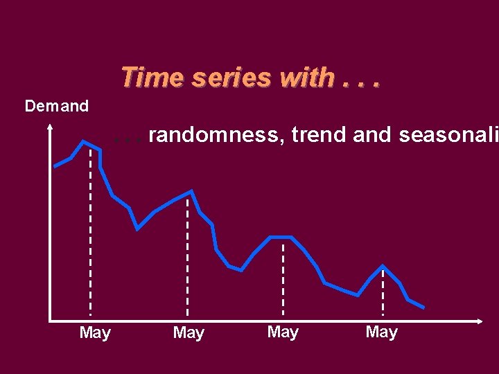
Time series with. . . Demand . . . randomness, trend and seasonali May May

Demand Forms of Forecast Movement Random movement Time (b) Cycle Demand Time (a) Trend Time (c) Seasonal pattern Time (d) Trend with seasonal pattern

Forms of Forecast Movement Irregular variation Trend Cycles 90 89 88 Seasonal variations

Idea Behind Time Series Models Distinguish between random fluctuations and true changes in underlying demand patterns.

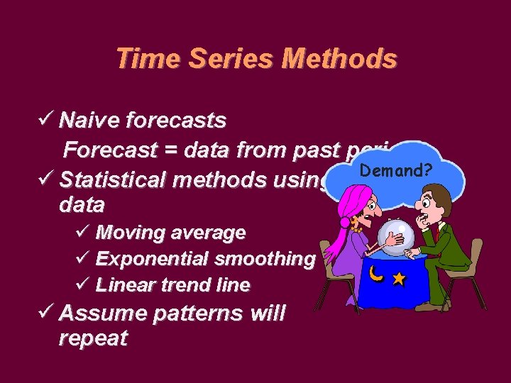
Time Series Methods ü Naive forecasts Forecast = data from past period Demand? ü Statistical methods using historical data ü Moving average ü Exponential smoothing ü Linear trend line ü Assume patterns will repeat

Naive Forecasts Uh, give me a minute. . We sold 250 wheels last week. . Now, next week we should sell. . The forecast for any period equals the previous period’s actual value.

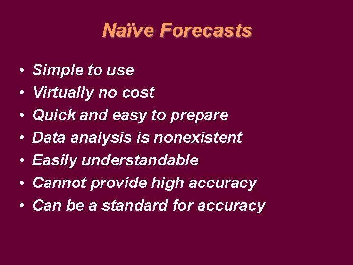
Naïve Forecasts • • Simple to use Virtually no cost Quick and easy to prepare Data analysis is nonexistent Easily understandable Cannot provide high accuracy Can be a standard for accuracy

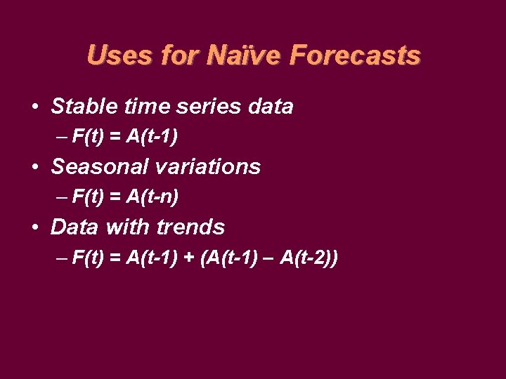
Uses for Naïve Forecasts • Stable time series data – F(t) = A(t-1) • Seasonal variations – F(t) = A(t-n) • Data with trends – F(t) = A(t-1) + (A(t-1) – A(t-2))

Techniques for Averaging • Moving Average • Weighted Moving Average • Exponential Smoothing Averaging techniques smooth fluctuations in a time series.

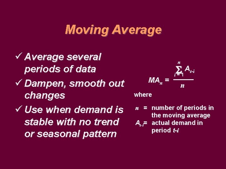
Moving Average ü Average several periods of data ü Dampen, smooth out changes ü Use when demand is stable with no trend or seasonal pattern n MAn = At-i i=1 n where n = number of periods in the moving average At-i= actual demand in period t-i

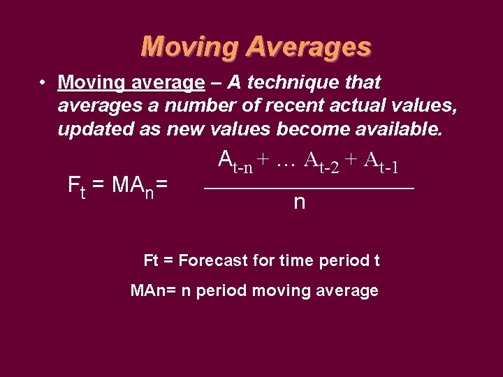
Moving Averages • Moving average – A technique that averages a number of recent actual values, updated as new values become available. Ft = MAn= At-n + … At-2 + At-1 n Ft = Forecast for time period t MAn= n period moving average

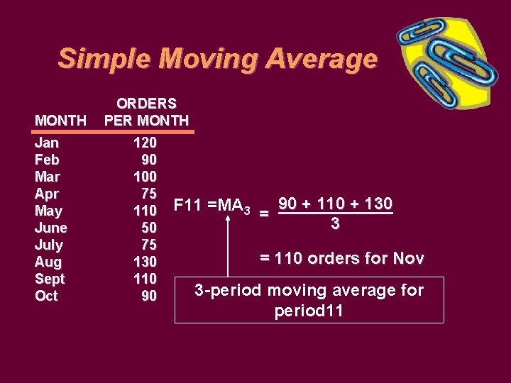
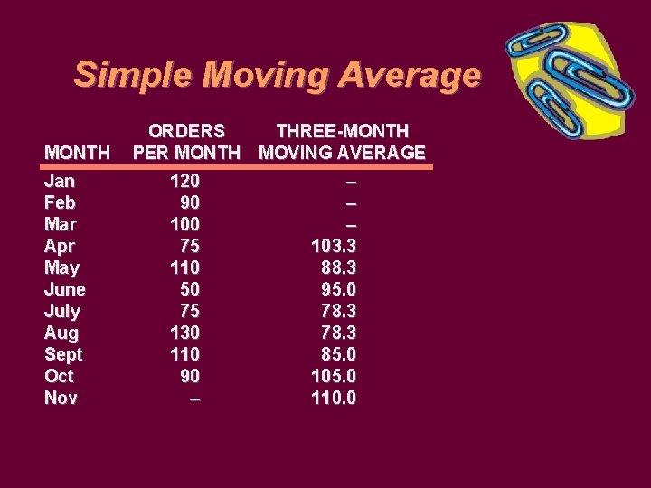
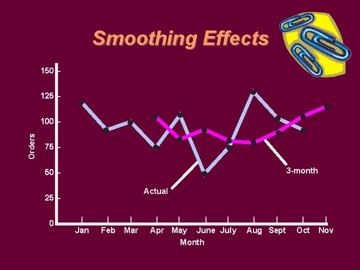
Simple Moving Average MONTH Jan Feb Mar Apr May June July Aug Sept Oct ORDERS PER MONTH 120 90 100 75 110 50 75 130 110 90 F 11 =MA 3 90 + 110 + 130 = 3 = 110 orders for Nov 3 -period moving average for period 11

Simple Moving Average MONTH Jan Feb Mar Apr May June July Aug Sept Oct Nov ORDERS THREE-MONTH PER MONTH MOVING AVERAGE 120 90 100 75 110 50 75 130 110 90 – – 103. 3 88. 3 95. 0 78. 3 85. 0 105. 0 110. 0

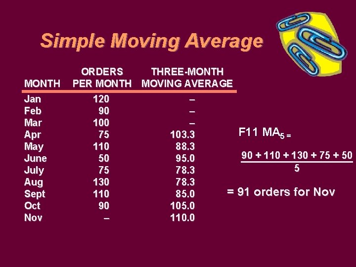
Simple Moving Average MONTH Jan Feb Mar Apr May June July Aug Sept Oct Nov ORDERS THREE-MONTH PER MONTH MOVING AVERAGE 120 90 100 75 110 50 75 130 110 90 – – 103. 3 88. 3 95. 0 78. 3 85. 0 105. 0 110. 0 F 11 MA 5 = 90 + 110 + 130 + 75 + 50 5 = 91 orders for Nov

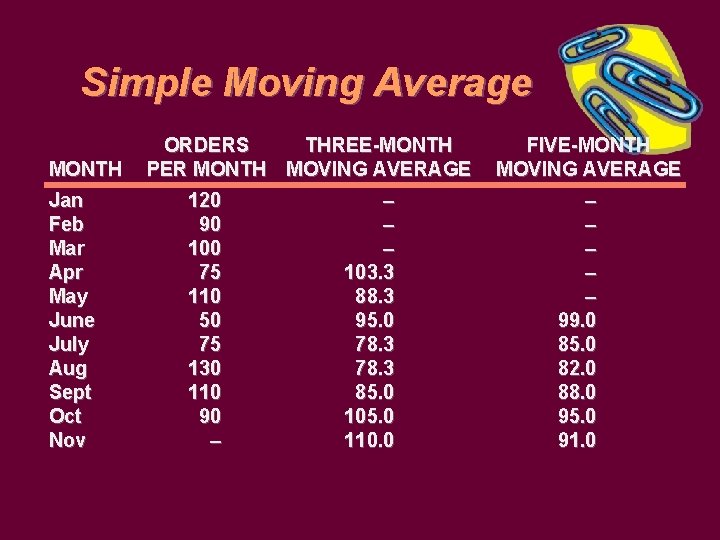
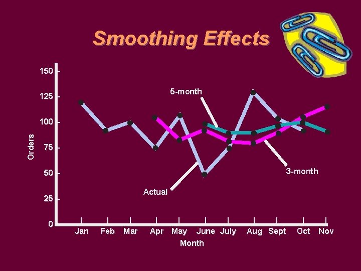
Simple Moving Average MONTH Jan Feb Mar Apr May June July Aug Sept Oct Nov ORDERS THREE-MONTH PER MONTH MOVING AVERAGE 120 90 100 75 110 50 75 130 110 90 – – 103. 3 88. 3 95. 0 78. 3 85. 0 105. 0 110. 0 FIVE-MONTH MOVING AVERAGE – – – 99. 0 85. 0 82. 0 88. 0 95. 0 91. 0

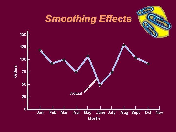
Smoothing Effects 150 – 125 – Orders 100 – 75 – 50 – Actual 25 – 0– | Jan | Feb | Mar | | Apr May June July Month | | Aug Sept | Oct | Nov

Smoothing Effects 150 – 125 – Orders 100 – 75 – 3 -month 50 – Actual 25 – 0– | Jan | Feb | Mar | | Apr May June July Month | | Aug Sept | Oct | Nov

Smoothing Effects 150 – 5 -month 125 – Orders 100 – 75 – 3 -month 50 – Actual 25 – 0– | Jan | Feb | Mar | | Apr May June July Month | | Aug Sept | Oct | Nov

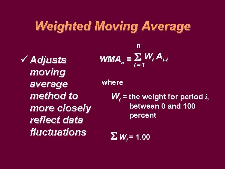
Weighted Moving Average n WMAn = Wi At-i ü Adjusts i=1 moving where average Wi = the weight for period i, method to between 0 and 100 more closely percent reflect data fluctuations W = 1. 00 i

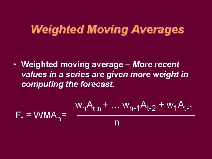
Weighted Moving Averages • Weighted moving average – More recent values in a series are given more weight in computing the forecast. Ft = WMAn= wn. At-n + … wn-1 At-2 + w 1 At-1 n

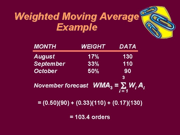
Weighted Moving Average Example MONTH August September October WEIGHT DATA 17% 33% 50% 130 110 90 3 November forecast WMA 3 = W i Ai i=1 = (0. 50)(90) + (0. 33)(110) + (0. 17)(130) = 103. 4 orders

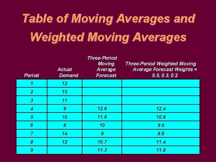
Table of Moving Averages and Weighted Moving Averages Period Actual Demand Three-Period Moving Average Forecast Three-Period Weighted Moving Average Forecast Weights = 0. 5, 0. 3, 0. 2 1 12 2 15 3 11 4 9 12. 6 12. 4 5 10 11. 6 10. 8 6 8 10 9. 9 7 14 9 8. 8 8 12 10. 7 11. 4 11. 3 11. 8 9

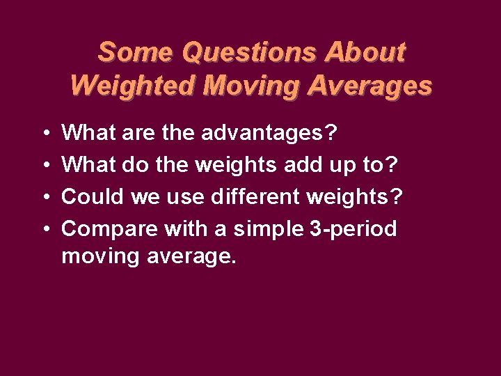
Some Questions About Weighted Moving Averages • • What are the advantages? What do the weights add up to? Could we use different weights? Compare with a simple 3 -period moving average.

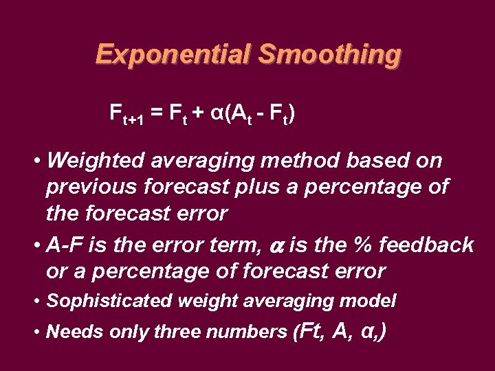
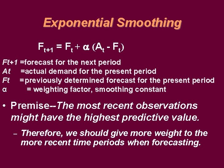
Exponential Smoothing Ft+1 = Ft + α(At - Ft) • Weighted averaging method based on previous forecast plus a percentage of the forecast error • A-F is the error term, is the % feedback or a percentage of forecast error • Sophisticated weight averaging model • Needs only three numbers (Ft, A, α, )

Exponential Smoothing Ft+1 = Ft + (At - Ft) Ft+1 =forecast for the next period At =actual demand for the present period Ft = previously determined forecast for the present period α = weighting factor, smoothing constant • Premise--The most recent observations might have the highest predictive value. – Therefore, we should give more weight to the more recent time periods when forecasting.

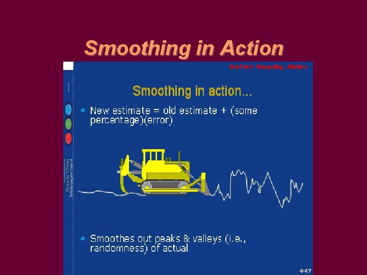
Smoothing in Action

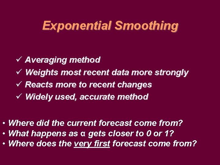
Exponential Smoothing ü Averaging method ü Weights most recent data more strongly ü Reacts more to recent changes ü Widely used, accurate method • Where did the current forecast come from? • What happens as α gets closer to 0 or 1? • Where does the very first forecast come from?

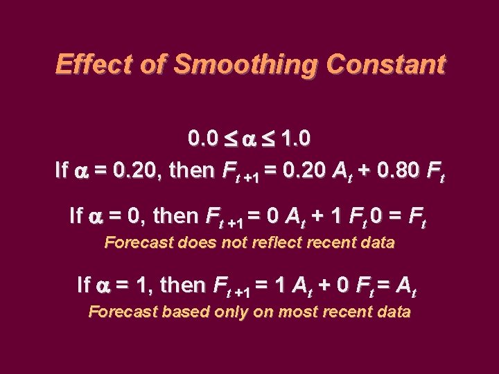
Effect of Smoothing Constant 0. 0 1. 0 If = 0. 20, then Ft +1 = 0. 20 At + 0. 80 Ft If = 0, then Ft +1 = 0 At + 1 Ft 0 = Ft Forecast does not reflect recent data If = 1, then Ft +1 = 1 At + 0 Ft = At Forecast based only on most recent data

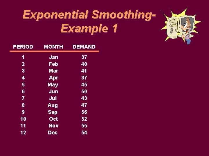
Exponential Smoothing. Example 1 PERIOD MONTH DEMAND 1 2 3 4 5 6 7 8 9 10 11 12 Jan Feb Mar Apr May Jun Jul Aug Sep Oct Nov Dec 37 40 41 37 45 50 43 47 56 52 55 54

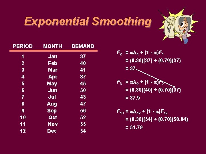
Exponential Smoothing PERIOD MONTH DEMAND 1 2 3 4 5 6 7 8 9 10 11 12 Jan Feb Mar Apr May Jun Jul Aug Sep Oct Nov Dec 37 40 41 37 45 50 43 47 56 52 55 54 F 2 = A 1 + (1 - )F 1 = (0. 30)(37) + (0. 70)(37) = 37 F 3 = A 2 + (1 - )F 2 = (0. 30)(40) + (0. 70)(37) = 37. 9 F 13 = A 12 + (1 - )F 12 = (0. 30)(54) + (0. 70)(50. 84) = 51. 79

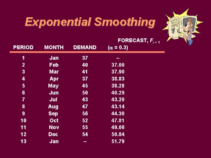
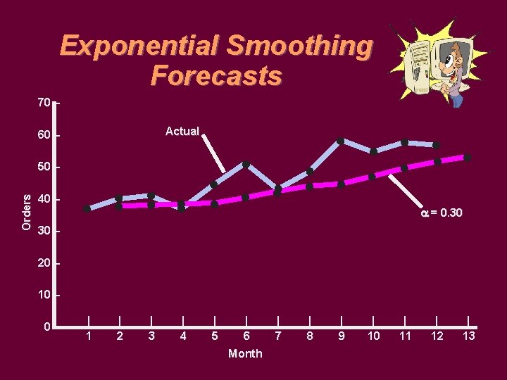
Exponential Smoothing PERIOD MONTH DEMAND 1 2 3 4 5 6 7 8 9 10 11 12 13 Jan Feb Mar Apr May Jun Jul Aug Sep Oct Nov Dec Jan 37 40 41 37 45 50 43 47 56 52 55 54 – FORECAST, Ft + 1 ( = 0. 3) – 37. 00 37. 90 38. 83 38. 28 40. 29 43. 20 43. 14 44. 30 47. 81 49. 06 50. 84 51. 79

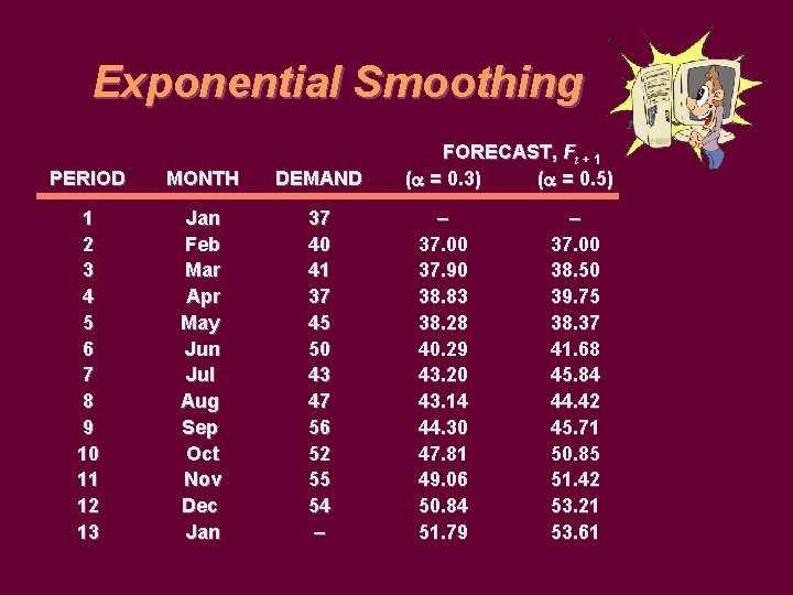
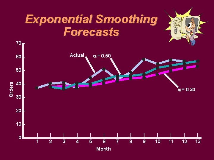
Exponential Smoothing PERIOD MONTH DEMAND 1 2 3 4 5 6 7 8 9 10 11 12 13 Jan Feb Mar Apr May Jun Jul Aug Sep Oct Nov Dec Jan 37 40 41 37 45 50 43 47 56 52 55 54 – FORECAST, Ft + 1 ( = 0. 3) ( = 0. 5) – 37. 00 37. 90 38. 83 38. 28 40. 29 43. 20 43. 14 44. 30 47. 81 49. 06 50. 84 51. 79 – 37. 00 38. 50 39. 75 38. 37 41. 68 45. 84 44. 42 45. 71 50. 85 51. 42 53. 21 53. 61

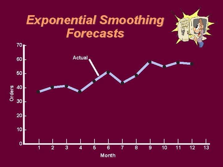
Exponential Smoothing Forecasts 70 – Actual 60 – Orders 50 – 40 – 30 – 20 – 10 – 0– | 1 | 2 | 3 | 4 | 5 | 6 Month | 7 | 8 | 9 | 10 | 11 | 12 | 13

Exponential Smoothing Forecasts 70 – Actual 60 – Orders 50 – 40 – = 0. 30 30 – 20 – 10 – 0– | 1 | 2 | 3 | 4 | 5 | 6 Month | 7 | 8 | 9 | 10 | 11 | 12 | 13

Exponential Smoothing Forecasts 70 – = 0. 50 Actual 60 – Orders 50 – 40 – = 0. 30 30 – 20 – 10 – 0– | 1 | 2 | 3 | 4 | 5 | 6 Month | 7 | 8 | 9 | 10 | 11 | 12 | 13

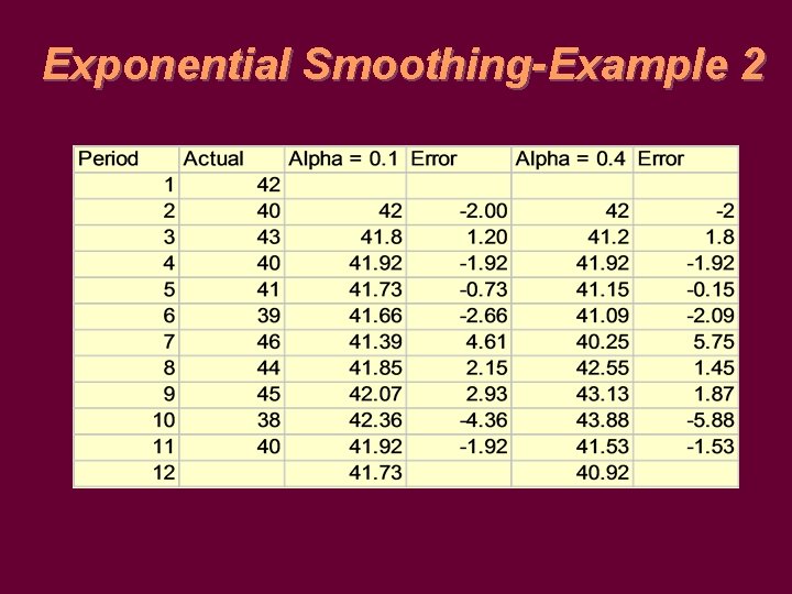
Exponential Smoothing-Example 2

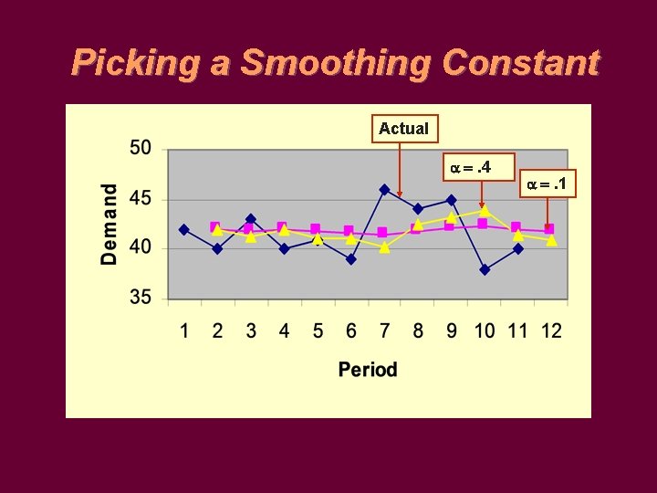
Picking a Smoothing Constant Actual . 4 . 1

Trends in Time Series Data What do you think will happen to a moving average or exponential smoothing model when there is a trend in the data?

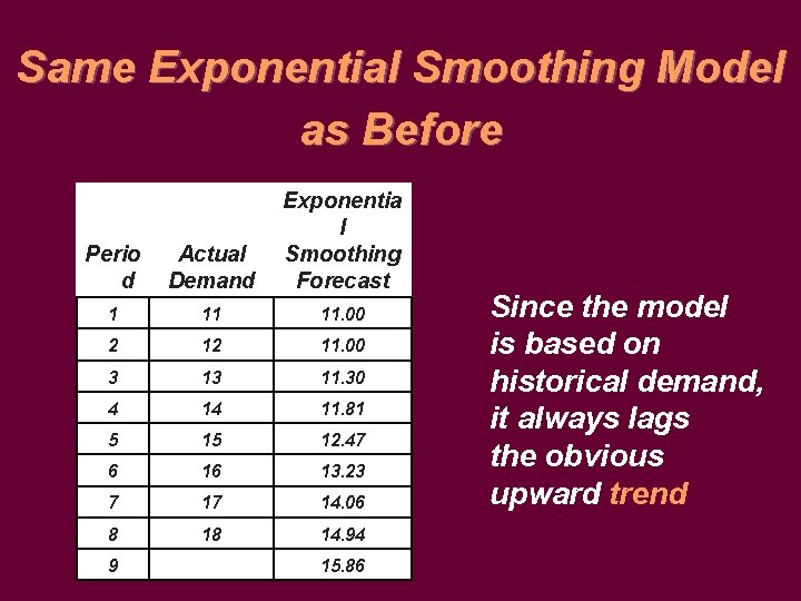
Same Exponential Smoothing Model as Before Perio d Actual Demand Exponentia l Smoothing Forecast 1 11 11. 00 2 12 11. 00 3 13 11. 30 4 14 11. 81 5 15 12. 47 6 16 13. 23 7 17 14. 06 8 18 14. 94 9 15. 86 Since the model is based on historical demand, it always lags the obvious upward trend

Trend-Adjusted Exponential Smoothing A variation of simple exponential smoothing can be used when a time series exhibits trend and it is called trend-adjusted exponential smoothing or double smoothing If a series exhibits trend, and simple smoothing is used on it the forecasts will all lag the trend: if the data are increasing, each forecast will be too low; if the data are decreasing, each forecast will be too high.

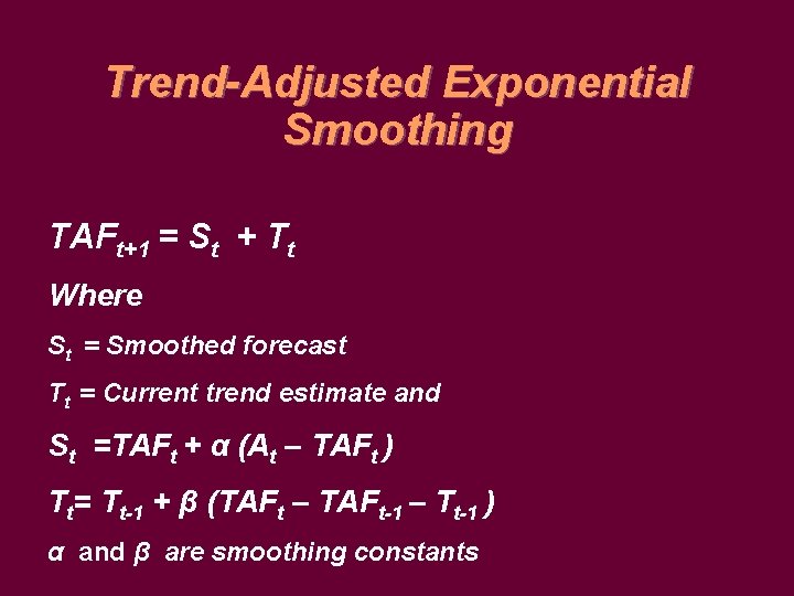
Trend-Adjusted Exponential Smoothing TAFt+1 = St + Tt Where St = Smoothed forecast Tt = Current trend estimate and St =TAFt + α (At – TAFt ) Tt= Tt-1 + β (TAFt – TAFt-1 – Tt-1 ) α and β are smoothing constants

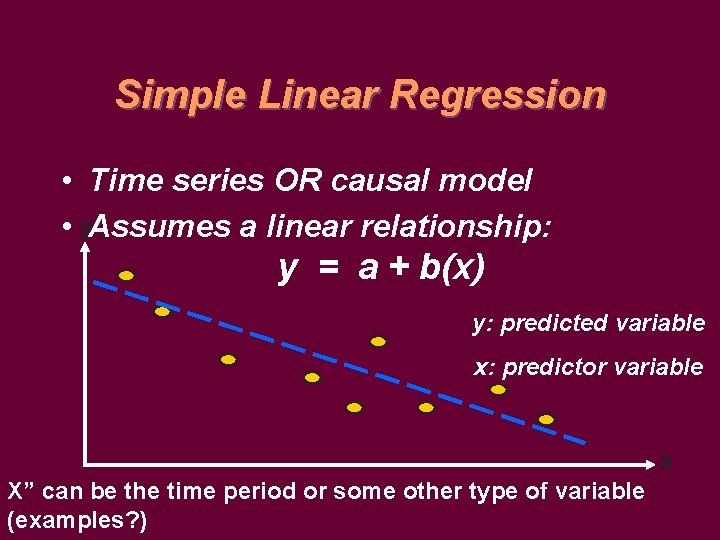
Simple Linear Regression • Time series OR causal model • y. Assumes a linear relationship: y = a + b(x) y: predicted variable x: predictor variable x X” can be the time period or some other type of variable (examples? )

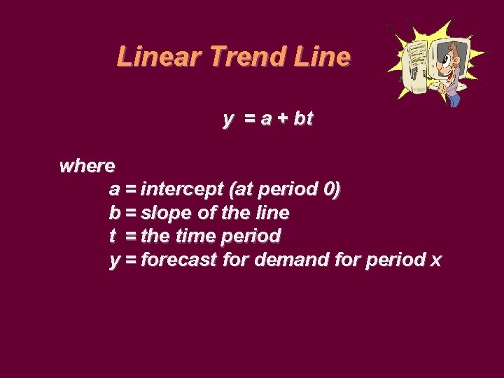
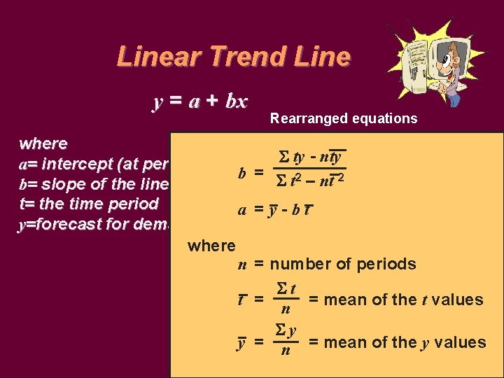
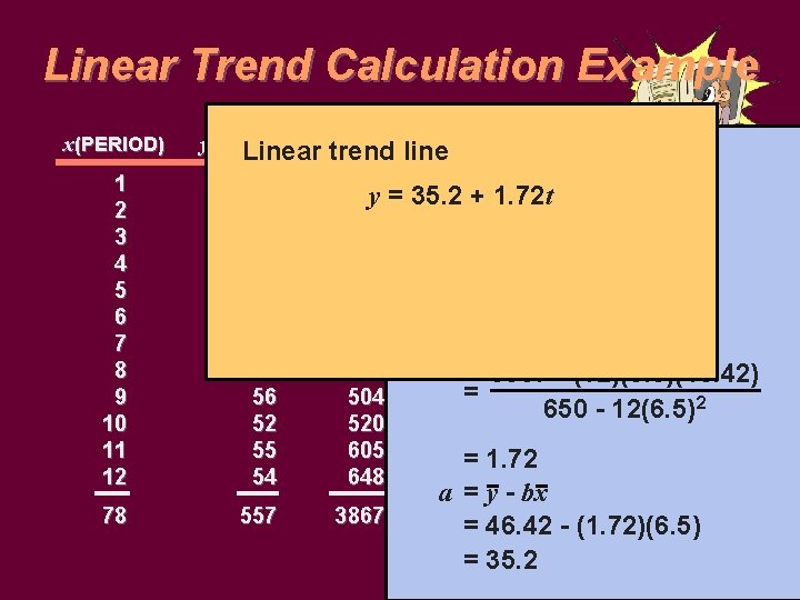
Linear Trend Line y = a + bt where a = intercept (at period 0) b = slope of the line t = the time period y = forecast for demand for period x

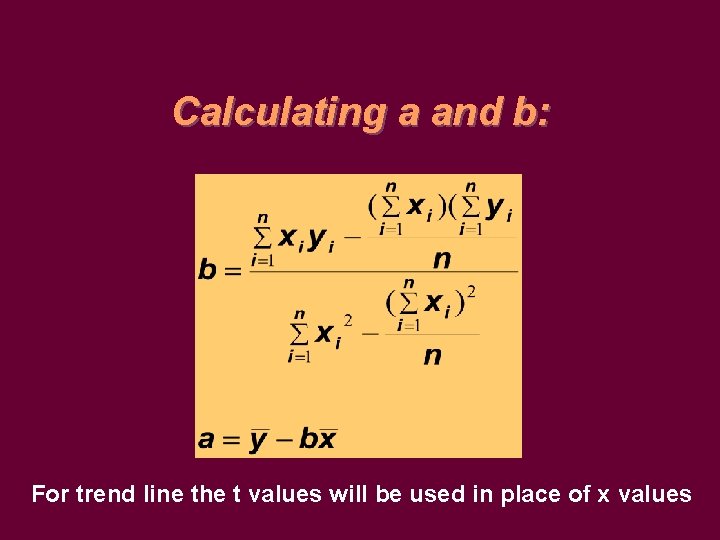
Calculating a and b: For trend line the t values will be used in place of x values

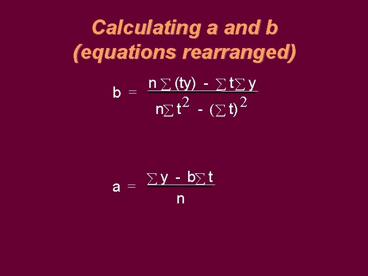
Calculating a and b (equations rearranged) n (ty) - t y b = n t 2 - ( t) 2 y - b t a = n

Linear Trend Line y = a + bx Rearranged equations where ty - nty a= intercept (at period 0) b = t 2 – nt 2 b= slope of the line t= the time period a = y-bt y=forecast for demand for period x where n = number of periods t t = n = mean of the t values y y = n = mean of the y values

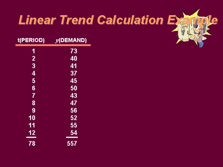
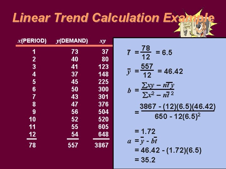
Linear Trend Calculation Example t(PERIOD) y(DEMAND) 1 2 3 4 5 6 7 8 9 10 11 12 73 40 41 37 45 50 43 47 56 52 55 54 78 557

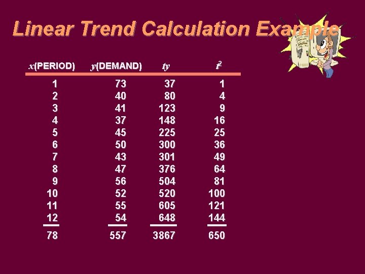
Linear Trend Calculation Example x(PERIOD) y(DEMAND) ty t 2 1 2 3 4 5 6 7 8 9 10 11 12 73 40 41 37 45 50 43 47 56 52 55 54 37 80 123 148 225 300 301 376 504 520 605 648 1 4 9 16 25 36 49 64 81 100 121 144 78 557 3867 650

Linear Trend Calculation Example x(PERIOD) y(DEMAND) xy 1 2 3 4 5 6 7 8 9 10 11 12 73 40 41 37 45 50 43 47 56 52 55 54 37 80 123 148 225 300 301 376 504 520 605 648 78 557 3867 x 2 78 t =1 = 6. 5 4 12 9 557 y 16 = = 46. 42 12 25 xy – nt y 36 b = 2 2 49 x – nt 64 3867 - (12)(6. 5)(46. 42) 81 = 650 - 12(6. 5)2 100 121 = 1. 72 144 a = y - bt 650 = 46. 42 - (1. 72)(6. 5) = 35. 2

Linear Trend Calculation Example x(PERIOD) y(DEMAND) Linear 1 2 3 4 5 6 7 8 9 10 11 12 73 40 41 37 45 50 43 47 56 52 55 54 78 557 2 xy line x trend 78 x = = 6. 5 37 y = 35. 2 +112 1. 72 t 80 4 557 123 9 y = = 46. 42 148 16 12 225 25 xy - nxy b =36 2 300 2 x nx 301 49 376 504 520 605 648 3867 643867 - (12)(6. 5)(46. 42) =81 650 - 12(6. 5)2 100 121 = 1. 72 144 a = y - bx 650 = 46. 42 - (1. 72)(6. 5) = 35. 2

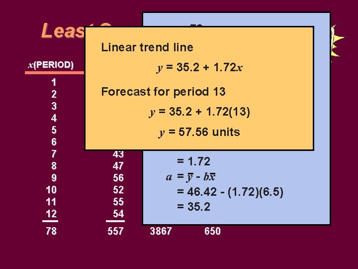
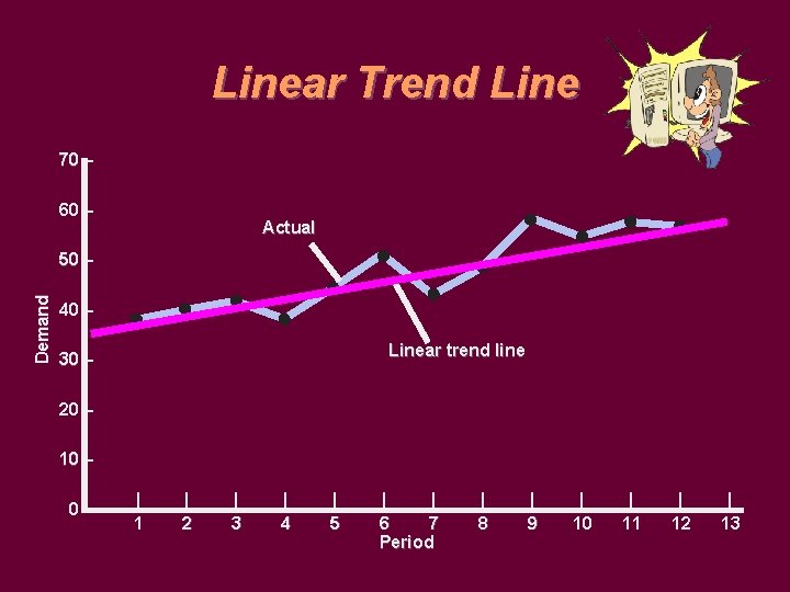
78 Least Squares x =Example = 6. 5 12 x(PERIOD) 1 2 3 4 5 6 7 8 9 10 11 12 78 Linear trend line 557 x 2 y(DEMAND) xy = = 46. 42 y y= 35. 2 12+ 1. 72 x 73 37 1 xy 13 - nxy Forecast for period 40 80 4 b = x 2 9 - nx 2 41 123 y 148 = 35. 2 + 1. 72(13) 37 386716 - (12)(6. 5)(46. 42) 45 225 y = =57. 56 25 units 650 - 12(6. 5)2 50 300 36 43 47 56 52 55 54 301 376 a 504 520 605 648 557 3867 = = 49 1. 7264 y - bx 81 10046. 42 121 35. 2 144 650 (1. 72)(6. 5)

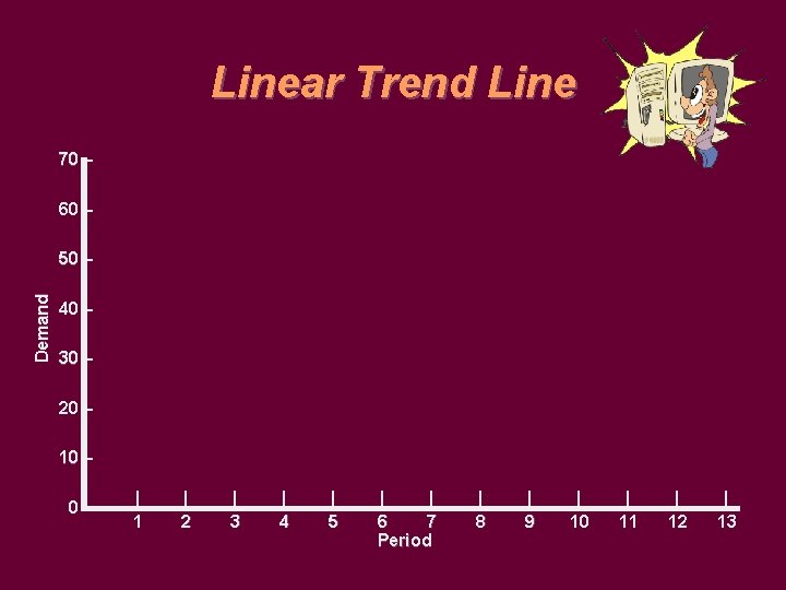
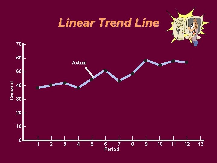
Linear Trend Line 70 – 60 – Demand 50 – 40 – 30 – 20 – 10 – 0– | 1 | 2 | 3 | 4 | 5 | | 6 7 Period | 8 | 9 | 10 | 11 | 12 | 13

Linear Trend Line 70 – 60 – Actual Demand 50 – 40 – 30 – 20 – 10 – 0– | 1 | 2 | 3 | 4 | 5 | | 6 7 Period | 8 | 9 | 10 | 11 | 12 | 13

Linear Trend Line 70 – 60 – Actual Demand 50 – 40 – Linear trend line 30 – 20 – 10 – 0– | 1 | 2 | 3 | 4 | 5 | | 6 7 Period | 8 | 9 | 10 | 11 | 12 | 13

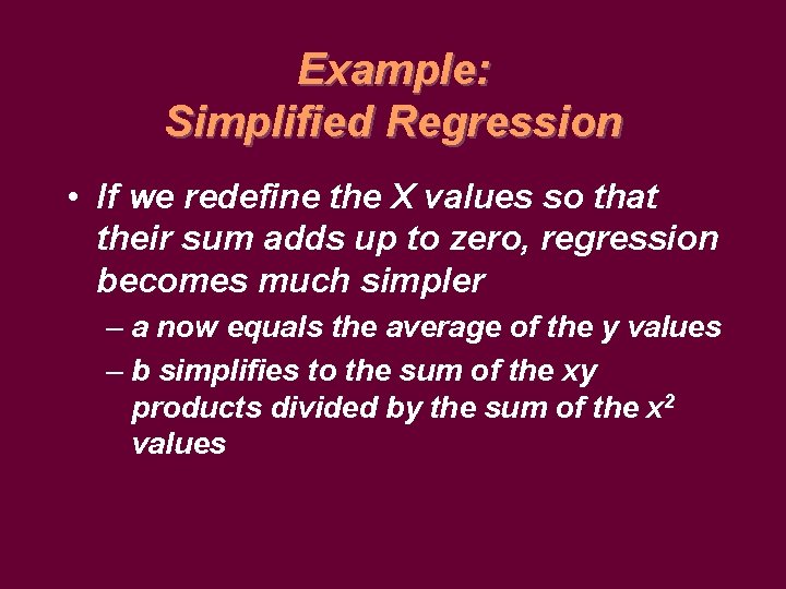
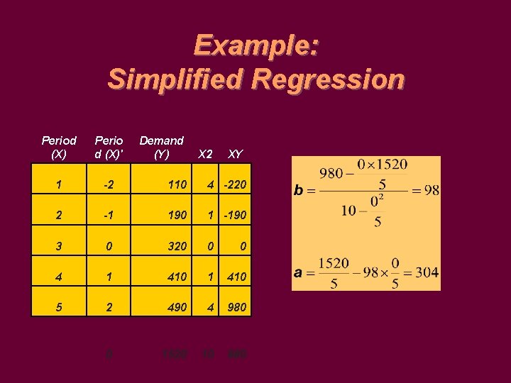
Example: Simplified Regression • If we redefine the X values so that their sum adds up to zero, regression becomes much simpler – a now equals the average of the y values – b simplifies to the sum of the xy products divided by the sum of the x 2 values

Example: Simplified Regression Period (X) Perio d (X)' Demand (Y) 1 -2 110 4 -220 2 -1 190 1 -190 3 0 320 0 0 4 1 410 5 2 490 4 980 0 1520 10 980 X 2 XY

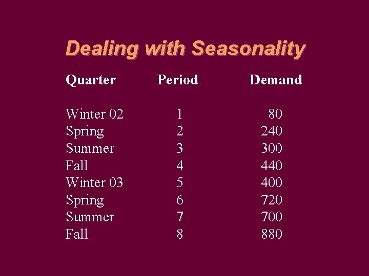
Dealing with Seasonality Quarter Period Winter 02 Spring Summer Fall Winter 03 Spring Summer Fall 1 2 3 4 5 6 7 8 Demand 80 240 300 440 400 720 700 880

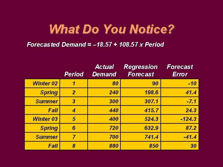
What Do You Notice? Forecasted Demand = – 18. 57 + 108. 57 x Period Actual Demand Regression Forecast Error Winter 02 1 80 90 -10 Spring 2 240 198. 6 41. 4 Summer 3 300 307. 1 -7. 1 Fall 4 440 415. 7 24. 3 Winter 03 5 400 524. 3 -124. 3 Spring 6 720 632. 9 87. 2 Summer 7 700 741. 4 -41. 4 Fall 8 880 850 30

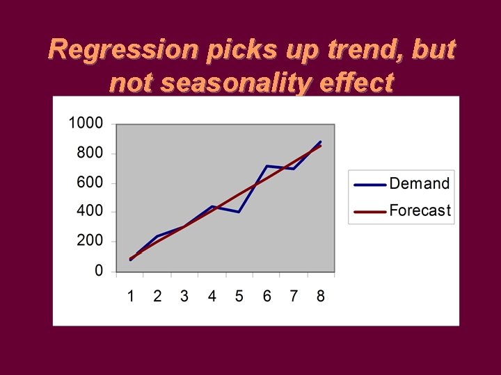
Regression picks up trend, but not seasonality effect

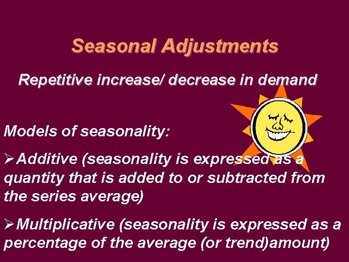
Seasonal Adjustments Repetitive increase/ decrease in demand Models of seasonality: ØAdditive (seasonality is expressed as a quantity that is added to or subtracted from the series average) ØMultiplicative (seasonality is expressed as a percentage of the average (or trend)amount)

Seasonal Adjustments ü The seasonal percentages in the multiplicative model are referred to as seasonal relatives or seasonal indexes

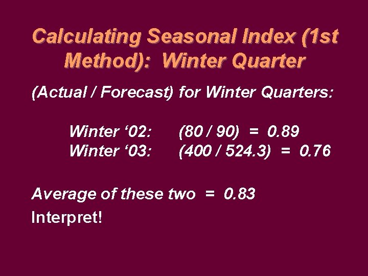
Calculating Seasonal Index (1 st Method): Winter Quarter (Actual / Forecast) for Winter Quarters: Winter ‘ 02: Winter ‘ 03: (80 / 90) = 0. 89 (400 / 524. 3) = 0. 76 Average of these two = 0. 83 Interpret!

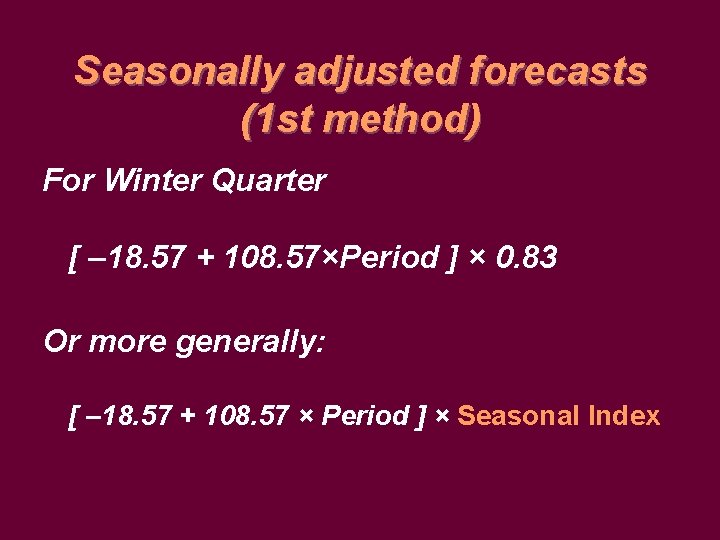
Seasonally adjusted forecasts (1 st method) For Winter Quarter [ – 18. 57 + 108. 57×Period ] × 0. 83 Or more generally: [ – 18. 57 + 108. 57 × Period ] × Seasonal Index

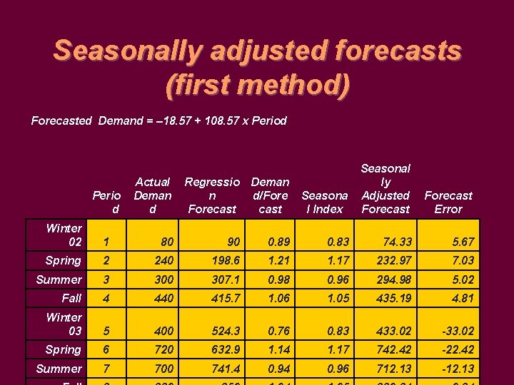
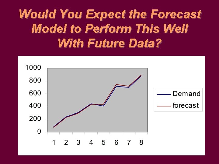
Seasonally adjusted forecasts (first method) Forecasted Demand = – 18. 57 + 108. 57 x Period Perio d Actual Deman d Regressio n Forecast Deman d/Fore cast Seasona l Index Seasonal ly Adjusted Forecast Error Winter 02 1 80 90 0. 89 0. 83 74. 33 5. 67 Spring 2 240 198. 6 1. 21 1. 17 232. 97 7. 03 Summer 3 300 307. 1 0. 98 0. 96 294. 98 5. 02 Fall 4 440 415. 7 1. 06 1. 05 435. 19 4. 81 Winter 03 5 400 524. 3 0. 76 0. 83 433. 02 -33. 02 Spring 6 720 632. 9 1. 14 1. 17 742. 42 -22. 42 Summer 7 700 741. 4 0. 96 712. 13 -12. 13

Would You Expect the Forecast Model to Perform This Well With Future Data?

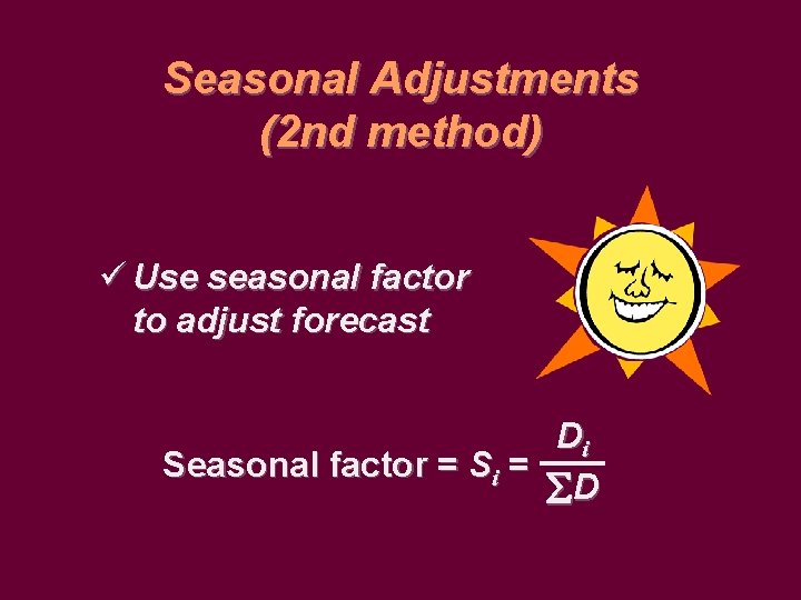
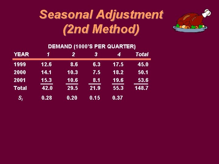
Seasonal Adjustments (2 nd method) ü Use seasonal factor to adjust forecast Di Seasonal factor = Si = D

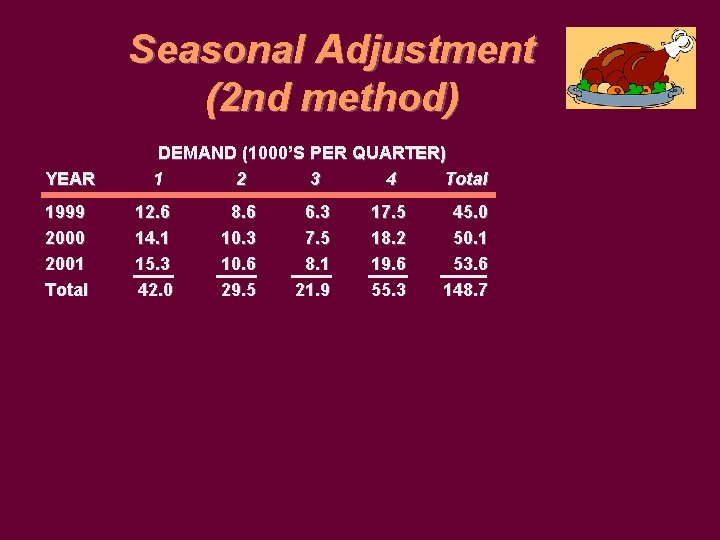
Seasonal Adjustment (2 nd method) YEAR 1999 2000 2001 Total DEMAND (1000’S PER QUARTER) 1 2 3 4 Total 12. 6 14. 1 15. 3 42. 0 8. 6 10. 3 10. 6 29. 5 6. 3 7. 5 8. 1 21. 9 17. 5 18. 2 19. 6 55. 3 45. 0 50. 1 53. 6 148. 7

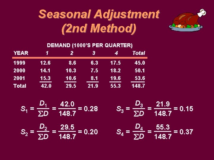
Seasonal Adjustment (2 nd Method) YEAR 1999 2000 2001 Total DEMAND (1000’S PER QUARTER) 1 2 3 4 Total 12. 6 14. 1 15. 3 42. 0 8. 6 10. 3 10. 6 29. 5 6. 3 7. 5 8. 1 21. 9 17. 5 18. 2 19. 6 55. 3 45. 0 50. 1 53. 6 148. 7 D 1 42. 0 S 1 = = = 0. 28 D 148. 7 D 3 21. 9 S 3 = = = 0. 15 D 148. 7 D 2 29. 5 S 2 = = = 0. 20 D 148. 7 D 4 55. 3 S 4 = = = 0. 37 D 148. 7

Seasonal Adjustment (2 nd Method) YEAR DEMAND (1000’S PER QUARTER) 1 2 3 4 Total 1999 2000 2001 Total 12. 6 14. 1 15. 3 42. 0 8. 6 10. 3 10. 6 29. 5 6. 3 7. 5 8. 1 21. 9 17. 5 18. 2 19. 6 55. 3 Si 0. 28 0. 20 0. 15 0. 37 45. 0 50. 1 53. 6 148. 7

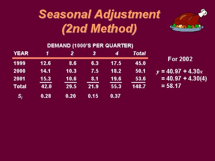
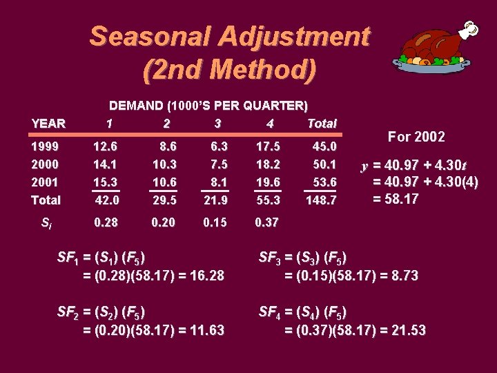
Seasonal Adjustment (2 nd Method) YEAR DEMAND (1000’S PER QUARTER) 1 2 3 4 Total 1999 2000 2001 Total 12. 6 14. 1 15. 3 42. 0 8. 6 10. 3 10. 6 29. 5 6. 3 7. 5 8. 1 21. 9 17. 5 18. 2 19. 6 55. 3 Si 0. 28 0. 20 0. 15 0. 37 45. 0 50. 1 53. 6 148. 7 For 2002 y = 40. 97 + 4. 30 x = 40. 97 + 4. 30(4) = 58. 17

Seasonal Adjustment (2 nd Method) YEAR DEMAND (1000’S PER QUARTER) 1 2 3 4 Total 1999 2000 2001 Total 12. 6 14. 1 15. 3 42. 0 8. 6 10. 3 10. 6 29. 5 6. 3 7. 5 8. 1 21. 9 17. 5 18. 2 19. 6 55. 3 Si 0. 28 0. 20 0. 15 0. 37 45. 0 50. 1 53. 6 148. 7 For 2002 y = 40. 97 + 4. 30 t = 40. 97 + 4. 30(4) = 58. 17 SF 1 = (S 1) (F 5) = (0. 28)(58. 17) = 16. 28 SF 3 = (S 3) (F 5) = (0. 15)(58. 17) = 8. 73 SF 2 = (S 2) (F 5) = (0. 20)(58. 17) = 11. 63 SF 4 = (S 4) (F 5) = (0. 37)(58. 17) = 21. 53

A Method for Computing Seasonal Relatives: Centered Moving Average Ø A commonly used method for representing the trend portion of a time series involves a centered moving average. Ø By virtue of its centered position it looks forward and looks backward, so it is able to closely follow data movements whether they involve trends, cycles, or random variability alone.

Computing Seasonal Relatives by Using Centered Moving Averages Ø The ratio of demand at period i to the centered average at period i is an estimate of the seasonal relative at that point.

Causal Models Time series assume that demand is a function of time. This is not always true. Sometimes it is possible to use the relationship between demand some other factor to develop forecast 1. Pounds of BBQ eaten at party. 2. Dollars spent on drought relief. 3. Lumber sales. Linear regression can be used in these situations as well.

Associative Forecasting Concepts: Predictor variables - used to predict values of variable interest Regression - technique for fitting a line to a set of points Least squares line - minimizes sum of squared deviations around the line

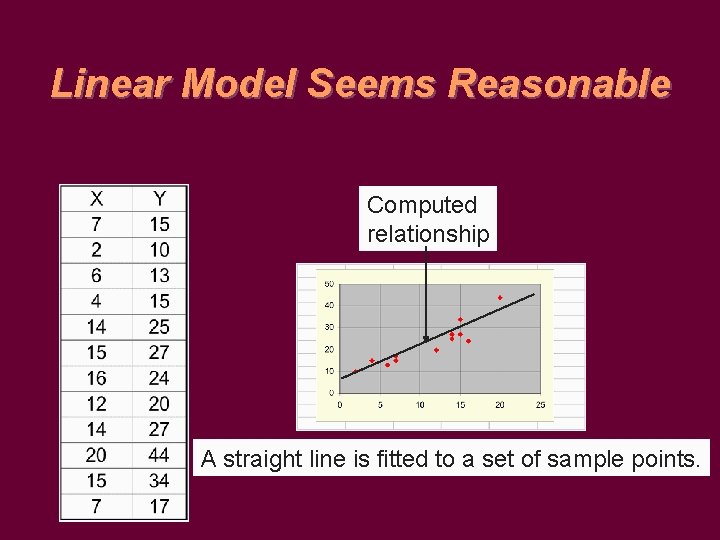
Causal Modeling with Linear Regression ü Study relationship between two or more variables ü Dependent variable y depends on independent variable x y = a + bx

Linear Model Seems Reasonable Computed relationship A straight line is fitted to a set of sample points.

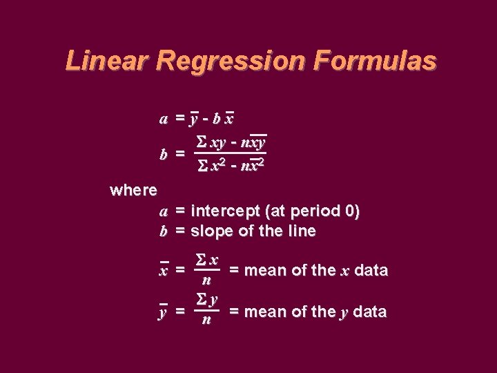
Linear Regression Formulas a = y-bx xy - nxy b = x 2 - nx 2 where a = intercept (at period 0) b = slope of the line x x = = mean of the x data n y y = n = mean of the y data

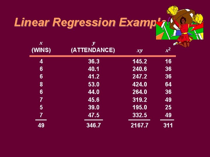
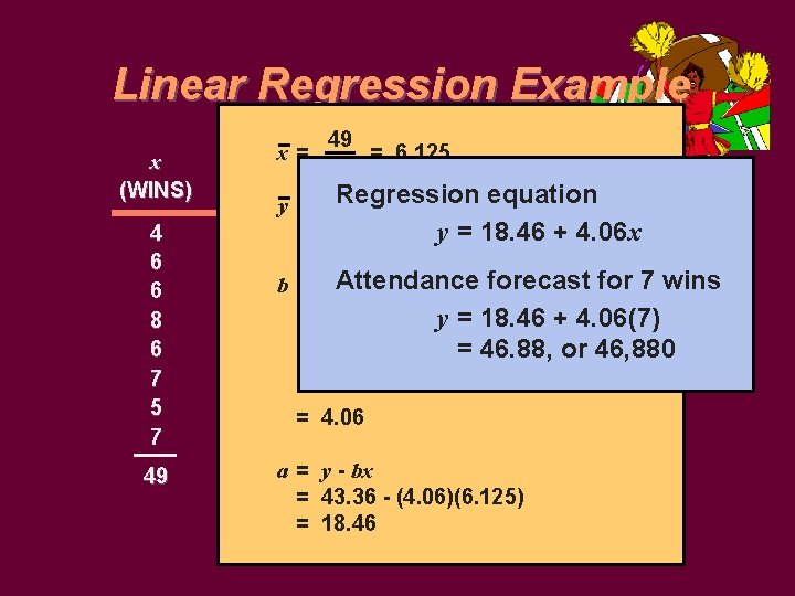
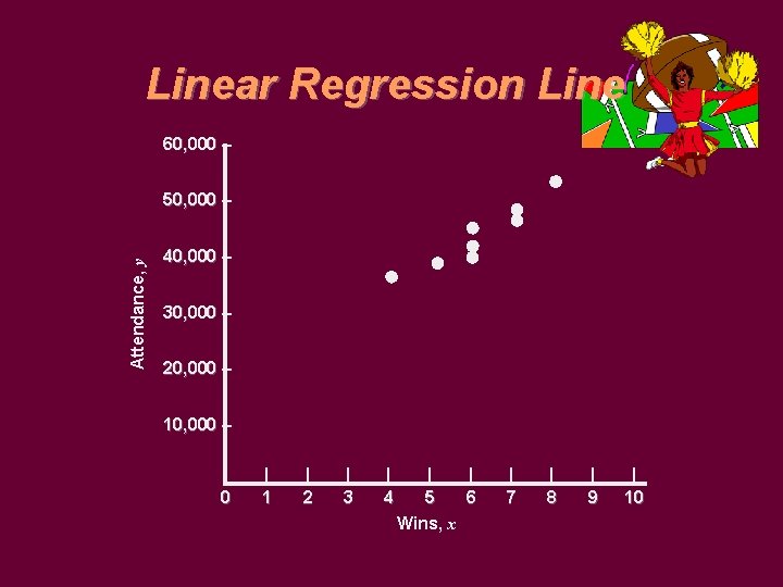
Linear Regression Example x (WINS) y (ATTENDANCE) xy x 2 4 6 6 8 6 7 5 7 36. 3 40. 1 41. 2 53. 0 44. 0 45. 6 39. 0 47. 5 145. 2 240. 6 247. 2 424. 0 264. 0 319. 2 195. 0 332. 5 16 36 36 64 36 49 25 49 49 346. 7 2167. 7 311

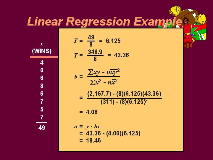
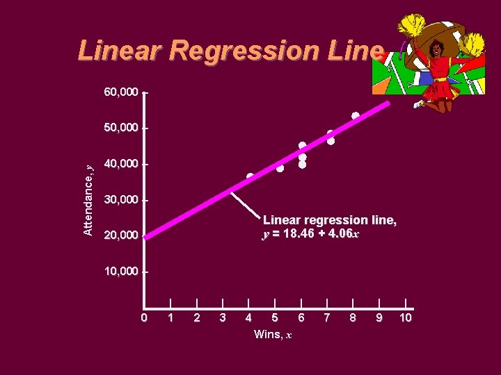
Linear Regression Example x (WINS) 4 6 6 8 6 7 5 7 49 49 = 6. 125 8 y (ATTENDANCE) xy x 2 346. 9 y= = 43. 36 8 36. 3 145. 2 16 40. 1 - nxy 2 240. 6 36 xy b = 41. 2 247. 2 36 2 2 x - nx 53. 0 424. 0 64 (2, 167. 7) - (8)(6. 125)(43. 36) 44. 0 264. 0 36 = 2 45. 6(311) - (8)(6. 125) 319. 2 49 39. 0 195. 0 25 = 4. 06 47. 5 332. 5 49 a = y 346. 7 - bx 2167. 7 311 = 43. 36 - (4. 06)(6. 125) = 18. 46 x=

Linear Regression Example x (WINS) 4 6 6 8 6 7 5 7 49 49 = 6. 125 8 y (ATTENDANCE) xy x 2 346. 9 Regression equation y= = 43. 36 8 36. 3 145. 2+ 4. 06 x 16 y = 18. 46 40. 1 - nxy 2 240. 6 36 xy Attendance forecast for 367 wins b = 41. 2 247. 2 2 - nx 2 x y = 18. 46 53. 0 424. 0+ 4. 06(7) 64 (2, 167. 7) - (8)(6. 125)(43. 36) 44. 0 264. 0 or 46, 880 36 = 46. 88, = 2 45. 6(311) - (8)(6. 125) 319. 2 49 39. 0 195. 0 25 = 4. 06 47. 5 332. 5 49 a = y 346. 7 - bx 2167. 7 311 = 43. 36 - (4. 06)(6. 125) = 18. 46 x=

Linear Regression Line 60, 000 – Attendance, y 50, 000 – 40, 000 – 30, 000 – 20, 000 – 10, 000 – | 0 | 1 | 2 | 3 | 4 | | 5 6 Wins, x | 7 | 8 | 9 | 10

Linear Regression Line 60, 000 – Attendance, y 50, 000 – 40, 000 – 30, 000 – Linear regression line, y = 18. 46 + 4. 06 x 20, 000 – 10, 000 – | 0 | 1 | 2 | 3 | 4 | | 5 6 Wins, x | 7 | 8 | 9 | 10

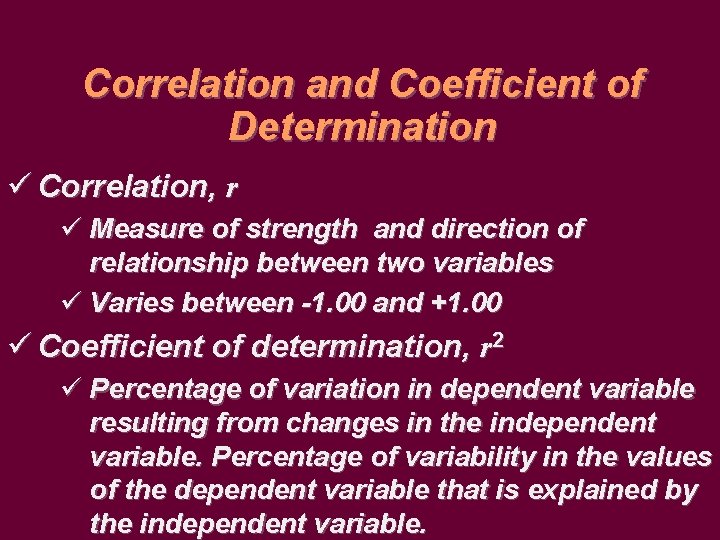
Correlation and Coefficient of Determination ü Correlation, r ü Measure of strength and direction of relationship between two variables ü Varies between -1. 00 and +1. 00 ü Coefficient of determination, r 2 ü Percentage of variation in dependent variable resulting from changes in the independent variable. Percentage of variability in the values of the dependent variable that is explained by the independent variable.

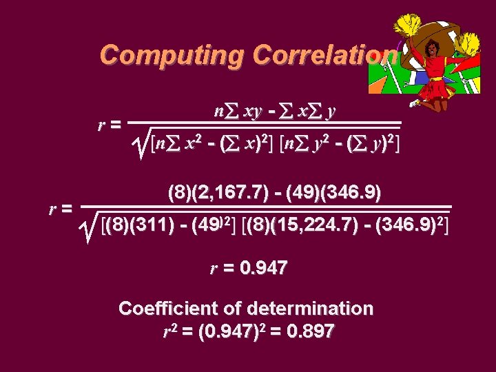
Computing Correlation r= r= n xy - x y [n x 2 - ( x)2] [n y 2 - ( y)2] (8)(2, 167. 7) - (49)(346. 9) [(8)(311) - (49)2] [(8)(15, 224. 7) - (346. 9)2] r = 0. 947 Coefficient of determination r 2 = (0. 947)2 = 0. 897

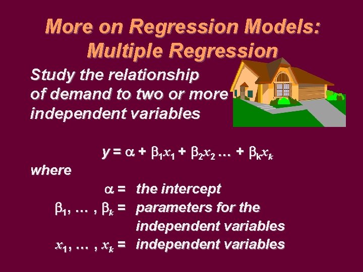
More on Regression Models: Multiple Regression Study the relationship of demand to two or more independent variables y = + 1 x 1 + 2 x 2 … + kxk where = the intercept 1, … , k = parameters for the independent variables x 1, … , xk = independent variables

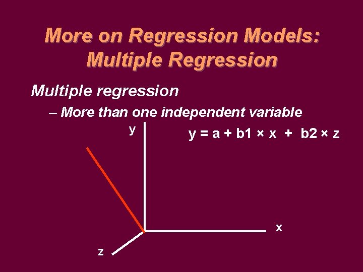
More on Regression Models: Multiple Regression Multiple regression – More than one independent variable y y = a + b 1 × x + b 2 × z x z

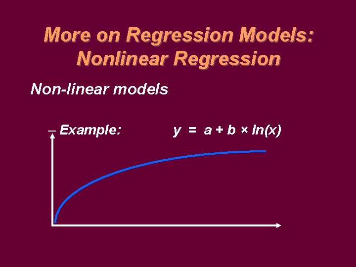
More on Regression Models: Nonlinear Regression Non-linear models – Example: y = a + b × ln(x)

Important Points in Using Regression Ø Always plot the data to verify that a linear relationship is appropriate Ø Check whether the data is timedependent. If so use time series instead of regression Ø A small correlation may imply that other variables are important

Measuring Forecast Accuracy How do we know: Ø If a forecast model is “best”? Ø If a forecast model is still working? Ø What types of errors a particular forecasting model is prone to make? We need measures of forecast accuracy

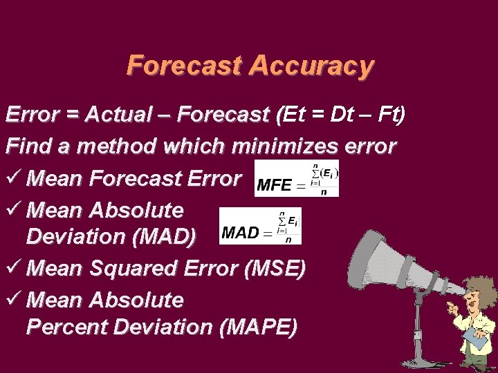
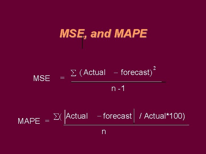
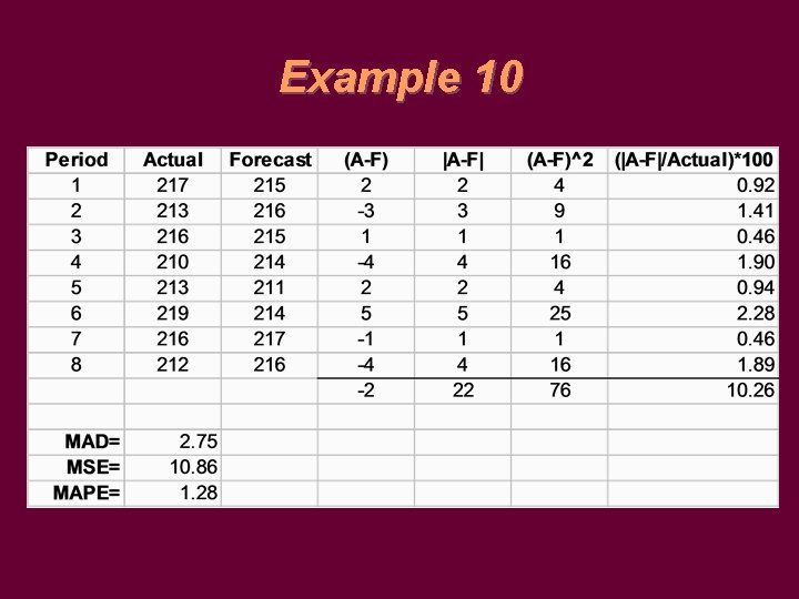
Forecast Accuracy Error = Actual – Forecast (Et = Dt – Ft) Find a method which minimizes error ü Mean Forecast Error ü Mean Absolute Deviation (MAD) ü Mean Squared Error (MSE) ü Mean Absolute Percent Deviation (MAPE)

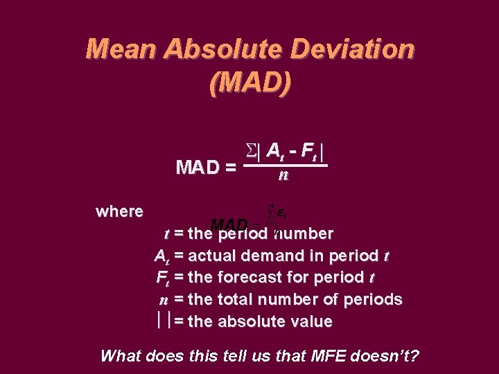
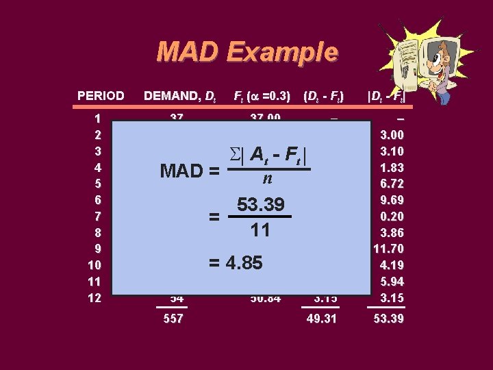
Mean Absolute Deviation (MAD) S At - F t MAD = n where t = the period number At = actual demand in period t Ft = the forecast for period t n = the total number of periods = the absolute value What does this tell us that MFE doesn’t?

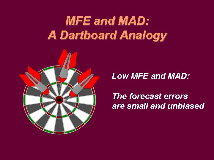
MFE and MAD: A Dartboard Analogy Low MFE and MAD: The forecast errors are small and unbiased

An Analogy Low MFE, but high MAD: On average, the arrows hit the bulls eye (so much for averages!)

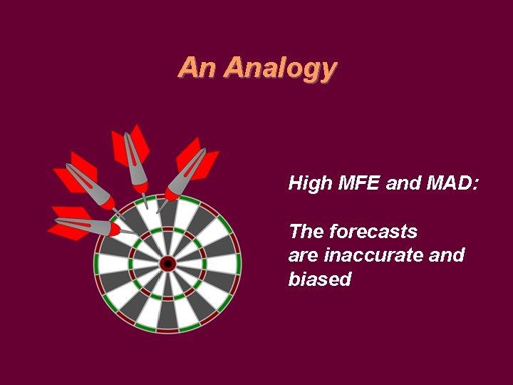
An Analogy High MFE and MAD: The forecasts are inaccurate and biased

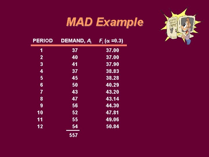
MAD Example PERIOD 1 2 3 4 5 6 7 8 9 10 11 12 DEMAND, At Ft ( =0. 3) 37 40 41 37 45 50 43 47 56 52 55 54 37. 00 37. 90 38. 83 38. 28 40. 29 43. 20 43. 14 44. 30 47. 81 49. 06 50. 84 557

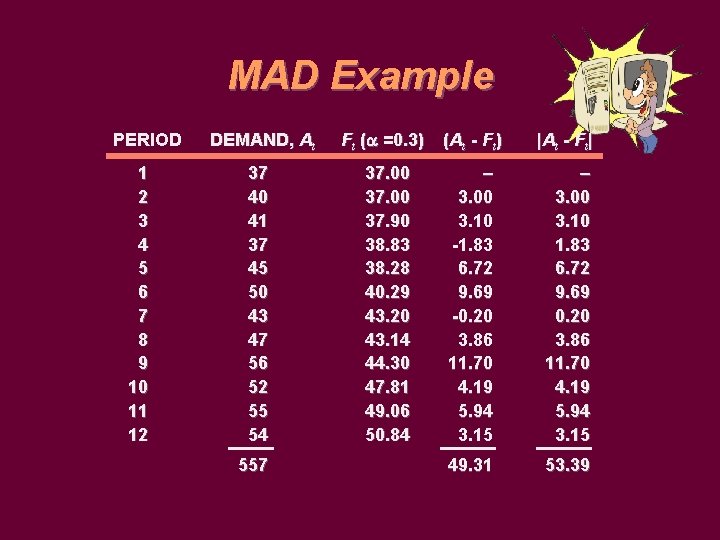
MAD Example PERIOD 1 2 3 4 5 6 7 8 9 10 11 12 DEMAND, At Ft ( =0. 3) (At - Ft) |At - Ft| 37 40 41 37 45 50 43 47 56 52 55 54 37. 00 37. 90 38. 83 38. 28 40. 29 43. 20 43. 14 44. 30 47. 81 49. 06 50. 84 – 3. 00 3. 10 -1. 83 6. 72 9. 69 -0. 20 3. 86 11. 70 4. 19 5. 94 3. 15 – 3. 00 3. 10 1. 83 6. 72 9. 69 0. 20 3. 86 11. 70 4. 19 5. 94 3. 15 49. 31 53. 39 557

MAD Example PERIOD 1 2 3 4 5 6 7 8 9 10 11 12 DEMAND, Dt 37 40 41 37 MAD 45 50 43 47 56 52 55 54 557 = = = Ft ( =0. 3) (Dt - Ft) |Dt - Ft| 37. 00 – 37. 00 3. 00 S 37. 90 At - Ft 3. 10 38. 83 -1. 83 n 38. 28 6. 72 40. 29 9. 69 53. 39 43. 20 -0. 20 11 43. 14 3. 86 44. 30 11. 70 47. 81 4. 19 4. 85 49. 06 5. 94 50. 84 3. 15 – 3. 00 3. 10 1. 83 6. 72 9. 69 0. 20 3. 86 11. 70 4. 19 5. 94 3. 15 49. 31 53. 39

MSE, and MAPE MSE = ( Actual forecast) 2 n -1 MAPE = ( Actual forecast / Actual*100) n

Example 10

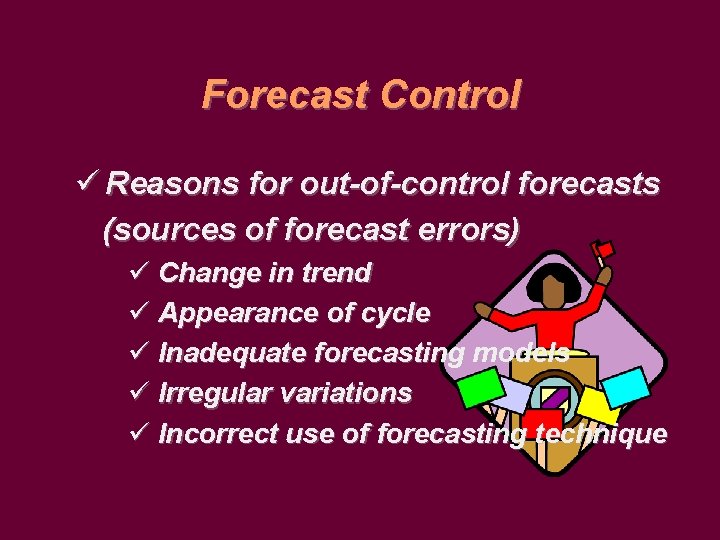
Forecast Control ü Reasons for out-of-control forecasts (sources of forecast errors) ü Change in trend ü Appearance of cycle ü Inadequate forecasting models ü Irregular variations ü Incorrect use of forecasting technique

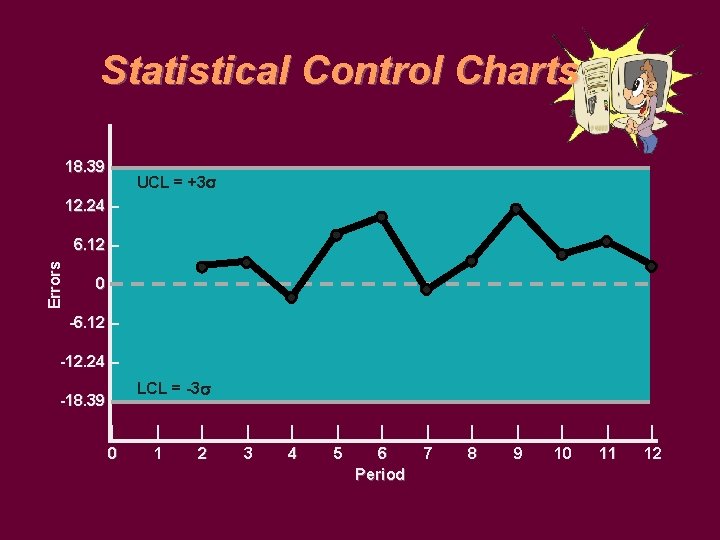
Controlling the Forecast A forecast is deemed to perform adequately when the errors exhibit only random variations • Control chart – A visual tool for monitoring forecast errors – Used to detect non-randomness in errors • Forecasting errors are in control if – All errors are within the control limits – No patterns, such as trends or cycles, are present

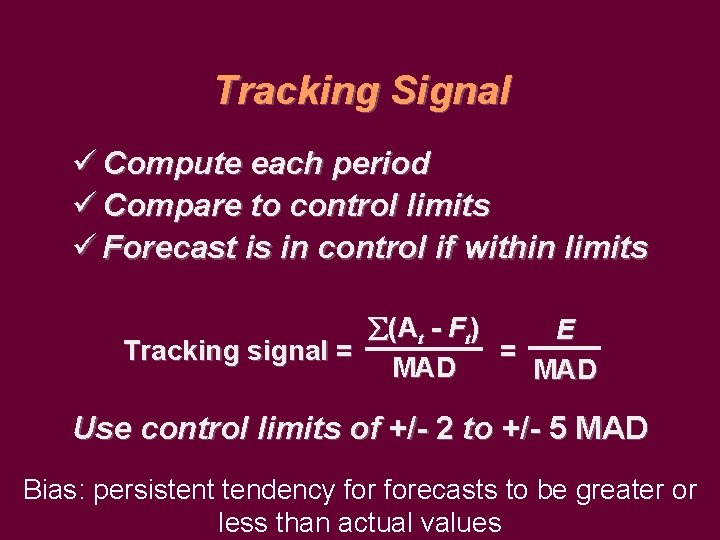
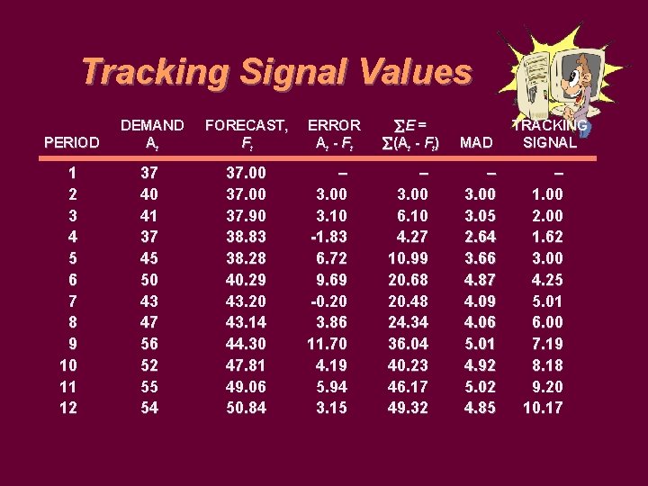
Tracking Signal ü Compute each period ü Compare to control limits ü Forecast is in control if within limits (A t - F t ) E Tracking signal = = MAD Use control limits of +/- 2 to +/- 5 MAD Bias: persistent tendency forecasts to be greater or less than actual values

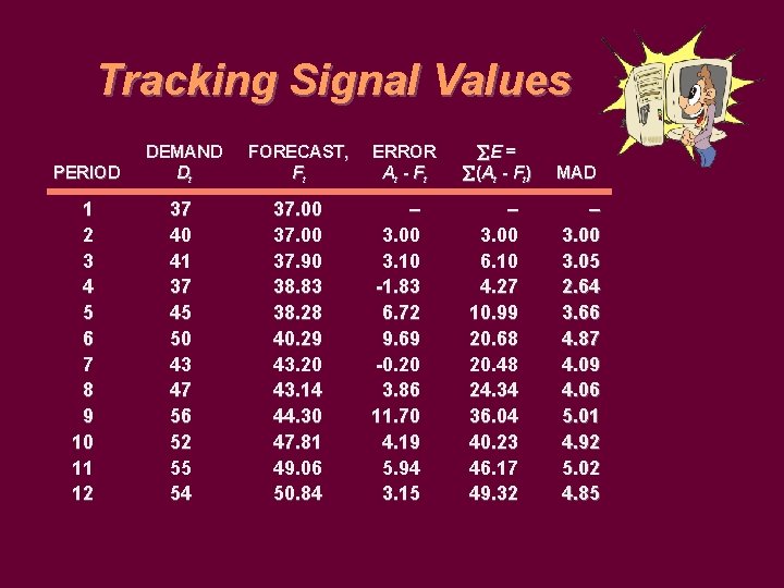
Tracking Signal Values PERIOD DEMAND Dt FORECAST, Ft 1 2 3 4 5 6 7 8 9 10 11 12 37 40 41 37 45 50 43 47 56 52 55 54 37. 00 37. 90 38. 83 38. 28 40. 29 43. 20 43. 14 44. 30 47. 81 49. 06 50. 84 ERROR At - F t – 3. 00 3. 10 -1. 83 6. 72 9. 69 -0. 20 3. 86 11. 70 4. 19 5. 94 3. 15 E = (At - Ft) MAD – 3. 00 6. 10 4. 27 10. 99 20. 68 20. 48 24. 34 36. 04 40. 23 46. 17 49. 32 – 3. 00 3. 05 2. 64 3. 66 4. 87 4. 09 4. 06 5. 01 4. 92 5. 02 4. 85

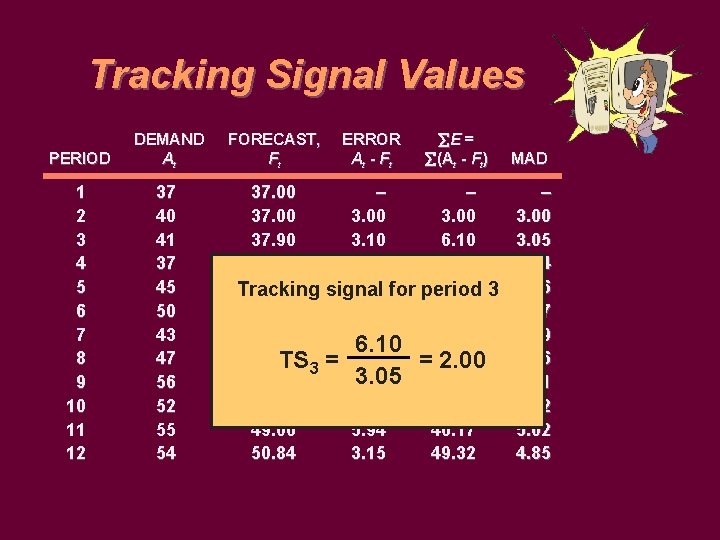
Tracking Signal Values PERIOD DEMAND At 1 2 3 4 5 6 7 8 9 10 11 12 37 40 41 37 45 50 43 47 56 52 55 54 FORECAST, Ft ERROR At - F t E = (At - Ft) 37. 00 – – 37. 00 37. 90 3. 10 6. 10 38. 83 -1. 83 4. 27 38. 28 6. 72 for period 10. 99 3 Tracking signal 40. 29 9. 69 20. 68 43. 20 -0. 20 6. 10 20. 48 43. 14 TS 3 = 3. 86 =24. 34 2. 00 3. 05 36. 04 44. 30 11. 70 47. 81 4. 19 40. 23 49. 06 5. 94 46. 17 50. 84 3. 15 49. 32 MAD – 3. 00 3. 05 2. 64 3. 66 4. 87 4. 09 4. 06 5. 01 4. 92 5. 02 4. 85

Tracking Signal Values PERIOD DEMAND At FORECAST, Ft 1 2 3 4 5 6 7 8 9 10 11 12 37 40 41 37 45 50 43 47 56 52 55 54 37. 00 37. 90 38. 83 38. 28 40. 29 43. 20 43. 14 44. 30 47. 81 49. 06 50. 84 ERROR At - F t – 3. 00 3. 10 -1. 83 6. 72 9. 69 -0. 20 3. 86 11. 70 4. 19 5. 94 3. 15 E = (At - Ft) MAD – 3. 00 6. 10 4. 27 10. 99 20. 68 20. 48 24. 34 36. 04 40. 23 46. 17 49. 32 – 3. 00 3. 05 2. 64 3. 66 4. 87 4. 09 4. 06 5. 01 4. 92 5. 02 4. 85 TRACKING SIGNAL – 1. 00 2. 00 1. 62 3. 00 4. 25 5. 01 6. 00 7. 19 8. 18 9. 20 10. 17

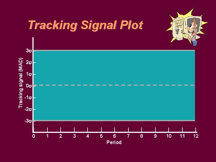
Tracking Signal Plot Tracking signal (MAD) 3 – 2 – 1 – 0 – -1 – -2 – -3 – | 0 | 1 | 2 | 3 | 4 | 5 | 6 Period | 7 | 8 | 9 | 10 | 11 | 12

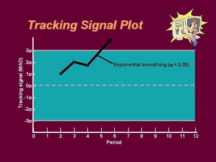
Tracking Signal Plot Tracking signal (MAD) 3 – 2 – Exponential smoothing ( = 0. 30) 1 – 0 – -1 – -2 – -3 – | 0 | 1 | 2 | 3 | 4 | 5 | 6 Period | 7 | 8 | 9 | 10 | 11 | 12

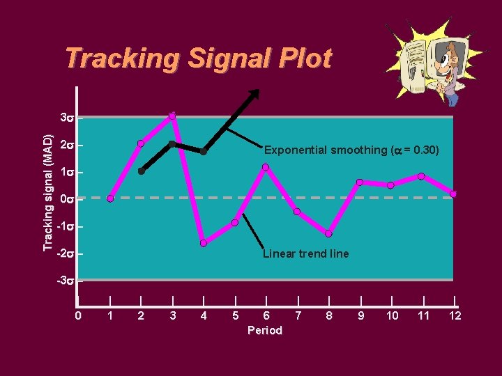
Tracking Signal Plot Tracking signal (MAD) 3 – 2 – Exponential smoothing ( = 0. 30) 1 – 0 – -1 – -2 – Linear trend line -3 – | 0 | 1 | 2 | 3 | 4 | 5 | 6 Period | 7 | 8 | 9 | 10 | 11 | 12

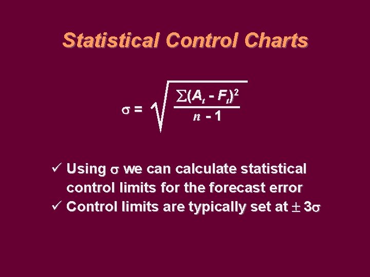
Statistical Control Charts = (A t - F t )2 n-1 ü Using we can calculate statistical control limits for the forecast error ü Control limits are typically set at 3

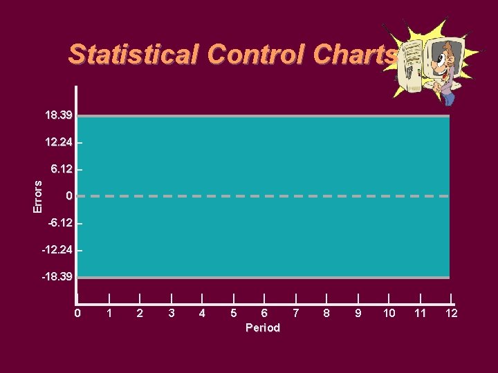
Statistical Control Charts 18. 39 – 12. 24 – Errors 6. 12 – 0– -6. 12 – -12. 24 – -18. 39 – | 0 | 1 | 2 | 3 | 4 | 5 | 6 Period | 7 | 8 | 9 | 10 | 11 | 12

Statistical Control Charts 18. 39 – UCL = +3 12. 24 – Errors 6. 12 – 0– -6. 12 – -12. 24 – -18. 39 – | 0 LCL = -3 | 1 | 2 | 3 | 4 | 5 | 6 Period | 7 | 8 | 9 | 10 | 11 | 12

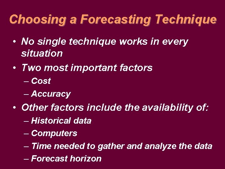
Choosing a Forecasting Technique • No single technique works in every situation • Two most important factors – Cost – Accuracy • Other factors include the availability of: – Historical data – Computers – Time needed to gather and analyze the data – Forecast horizon