Financial Analysis Planning and Forecasting Theory and Application

Financial Analysis, Planning and Forecasting Theory and Application Chapter 5 Determination and Applications of Nominal and Real Rates-Of-Return in Financial Analysis By Cheng F. Lee Rutgers University, USA John Lee Center for PBBEF Research, USA 1

Outline v v v v v 5. 1 5. 2 5. 3 Introduction Theoretical justification of paying interest Rate-of-return measurements and types of averages Discrete rates-of-return and continuous rates-of-return Types of averages Power means 5. 4 Theories of the term structure and their applications 5. 5 Interest rate, price-level changes, and components of risk premium Imperfect-foresight case Perfect-foresight case 5. 6 Three hypotheses about inflation and the value of the firm: a review The debtor-creditor hypothesis The tax-effects hypothesis Operating-income hypothesis The relationship among the three hypotheses 5. 7 Summary and concluding remarks Appendix 5 A. Compounding and discounting processes and their applications Appendix 5 B. Taylor-series expansion and its applications to rates-of-return determination 2

5. 3 Rates-of-return measurements and types of averages v v v Discrete rates-of-return and continuous rates-of-return Types of averages Power means 3

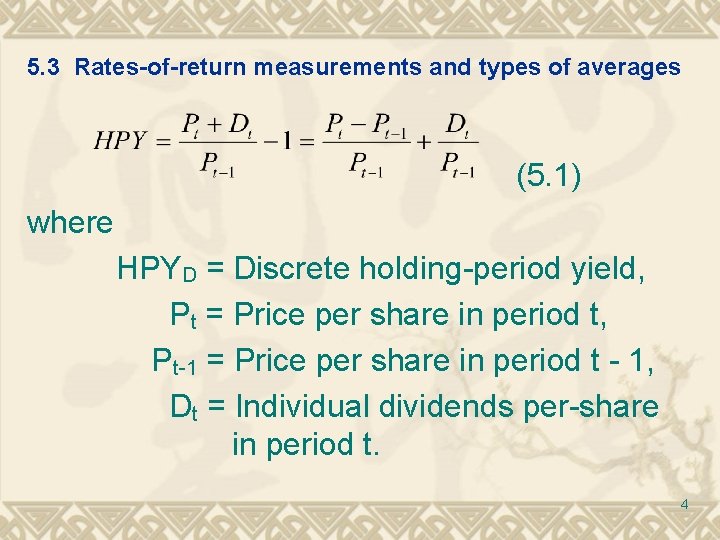
5. 3 Rates-of-return measurements and types of averages (5. 1) where HPYD = Discrete holding-period yield, Pt = Price per share in period t, Pt-1 = Price per share in period t - 1, Dt = Individual dividends per-share in period t. 4

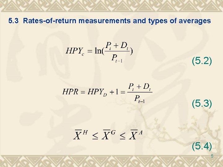
5. 3 Rates-of-return measurements and types of averages (5. 2) (5. 3) (5. 4) 5

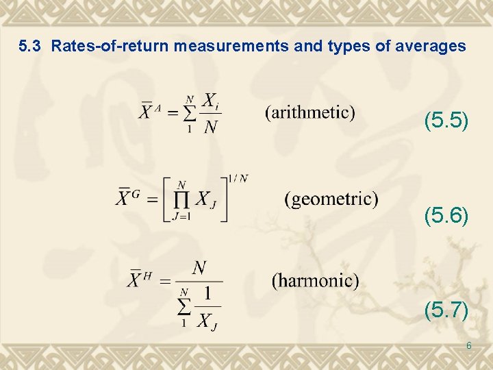
5. 3 Rates-of-return measurements and types of averages (5. 5) (5. 6) (5. 7) 6

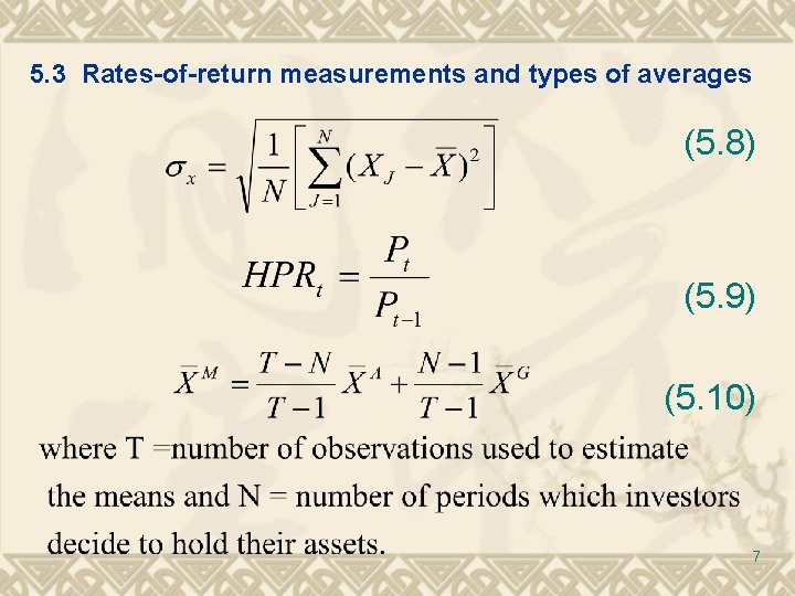
5. 3 Rates-of-return measurements and types of averages (5. 8) (5. 9) (5. 10) 7

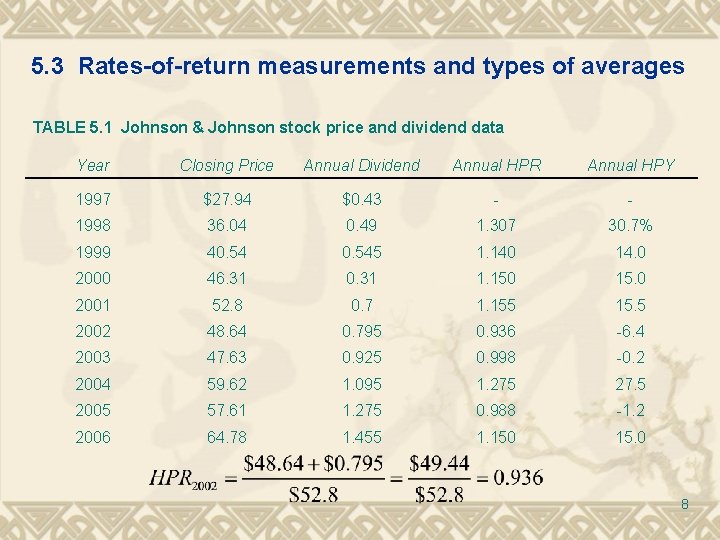
5. 3 Rates-of-return measurements and types of averages TABLE 5. 1 Johnson & Johnson stock price and dividend data Year Closing Price Annual Dividend Annual HPR Annual HPY 1997 $27. 94 $0. 43 - - 1998 36. 04 0. 49 1. 307 30. 7% 1999 40. 545 1. 140 14. 0 2000 46. 31 0. 31 1. 150 15. 0 2001 52. 8 0. 7 1. 155 15. 5 2002 48. 64 0. 795 0. 936 -6. 4 2003 47. 63 0. 925 0. 998 -0. 2 2004 59. 62 1. 095 1. 275 27. 5 2005 57. 61 1. 275 0. 988 -1. 2 2006 64. 78 1. 455 1. 150 15. 0 8

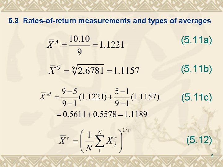
5. 3 Rates-of-return measurements and types of averages (5. 11 a) (5. 11 b) (5. 11 c) (5. 12) 9

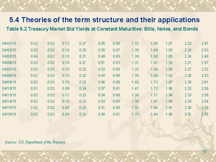
5. 4 Theories of the term structure and their applications Table 5. 2 Treasury Market Bid Yields at Constant Maturities: Bills, Notes, and Bonds 04/01/15 0. 02 0. 03 0. 12 0. 27 0. 55 0. 86 1. 32 1. 65 1. 87 2. 23 2. 47 04/02/15 0. 02 0. 10 0. 25 0. 55 0. 87 1. 35 1. 69 1. 92 2. 29 2. 53 04/03/15 0. 04 0. 02 0. 10 0. 21 0. 49 0. 80 1. 26 1. 60 1. 85 2. 24 2. 49 04/06/15 0. 02 0. 03 0. 10 0. 21 0. 51 0. 83 1. 31 1. 67 1. 92 2. 31 2. 57 04/07/15 0. 02 0. 10 0. 22 0. 52 0. 85 1. 32 1. 66 1. 89 2. 27 2. 52 04/08/15 0. 02 0. 03 0. 10 0. 22 0. 54 0. 86 1. 35 1. 68 1. 92 2. 28 2. 53 04/09/15 0. 02 0. 03 0. 10 0. 22 0. 56 0. 89 1. 40 1. 73 1. 97 2. 35 2. 61 04/10/15 0. 01 0. 02 0. 09 0. 24 0. 57 0. 91 1. 41 1. 73 1. 96 2. 33 2. 58 04/13/15 0. 02 0. 03 0. 11 0. 23 0. 54 0. 89 1. 38 1. 71 1. 94 2. 33 2. 58 04/14/15 0. 02 0. 10 0. 23 0. 53 0. 85 1. 34 1. 67 1. 90 2. 29 2. 54 04/15/15 0. 02 0. 08 0. 23 0. 51 0. 85 1. 33 1. 66 1. 91 2. 30 2. 55 04/16/15 0. 03 0. 02 0. 08 0. 22 0. 50 0. 81 1. 31 1. 64 1. 90 2. 31 2. 56 Sources: U. S. Department of the Treasury. 10

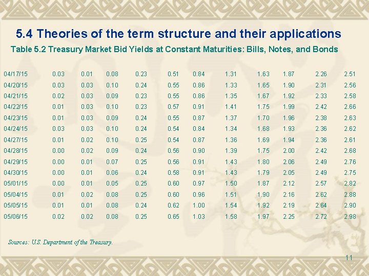
5. 4 Theories of the term structure and their applications Table 5. 2 Treasury Market Bid Yields at Constant Maturities: Bills, Notes, and Bonds 04/17/15 0. 03 0. 01 0. 08 0. 23 0. 51 0. 84 1. 31 1. 63 1. 87 2. 26 2. 51 04/20/15 0. 03 0. 10 0. 24 0. 55 0. 86 1. 33 1. 65 1. 90 2. 31 2. 56 04/21/15 0. 02 0. 03 0. 09 0. 23 0. 55 0. 86 1. 35 1. 67 1. 92 2. 33 2. 58 04/22/15 0. 01 0. 03 0. 10 0. 23 0. 57 0. 91 1. 41 1. 75 1. 99 2. 42 2. 66 04/23/15 0. 01 0. 03 0. 09 0. 24 0. 55 0. 87 1. 37 1. 70 1. 96 2. 38 2. 63 04/24/15 0. 03 0. 10 0. 24 0. 54 0. 84 1. 34 1. 68 1. 93 2. 36 2. 62 04/27/15 0. 01 0. 02 0. 10 0. 25 0. 54 0. 87 1. 36 1. 69 1. 94 2. 36 2. 61 04/28/15 0. 00 0. 02 0. 09 0. 24 0. 56 0. 90 1. 39 1. 75 2. 00 2. 42 2. 68 04/29/15 0. 00 0. 01 0. 07 0. 25 0. 56 0. 91 1. 43 1. 80 2. 06 2. 49 2. 76 04/30/15 0. 00 0. 01 0. 06 0. 24 0. 58 0. 91 1. 43 1. 79 2. 05 2. 49 2. 75 05/01/15 0. 00 0. 01 0. 05 0. 25 0. 60 0. 97 1. 50 1. 87 2. 12 2. 57 2. 82 05/04/15 0. 01 0. 02 0. 08 0. 25 0. 60 0. 96 1. 51 1. 90 2. 16 2. 62 2. 88 05/05/15 0. 01 0. 08 0. 24 0. 62 1. 00 1. 54 1. 92 2. 19 2. 64 2. 90 05/06/15 0. 02 0. 08 0. 25 0. 65 1. 03 1. 58 1. 97 2. 25 2. 72 2. 98 Sources: U. S. Department of the Treasury. 11

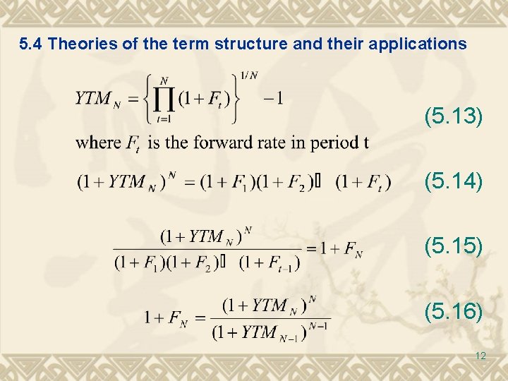
5. 4 Theories of the term structure and their applications (5. 13) (5. 14) (5. 15) (5. 16) 12

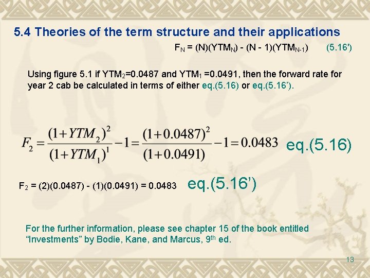
5. 4 Theories of the term structure and their applications FN = (N)(YTMN) - (N - 1)(YTMN-1) (5. 16′) Using figure 5. 1 if YTM 2=0. 0487 and YTM 1 =0. 0491, then the forward rate for year 2 cab be calculated in terms of either eq. (5. 16) or eq. (5. 16’). eq. (5. 16) F 2 = (2)(0. 0487) - (1)(0. 0491) = 0. 0483 eq. (5. 16’) For the further information, please see chapter 15 of the book entitled “Investments” by Bodie, Kane, and Marcus, 9 th ed. 13

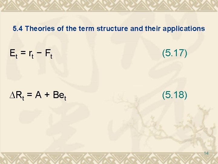
5. 4 Theories of the term structure and their applications E t = rt − F t (5. 17) ∆Rt = A + Bet (5. 18) 14

5. 5 Interest rate, price-level changes, and components of risk premium v v Imperfect-foresight case Perfect-foresight case 15

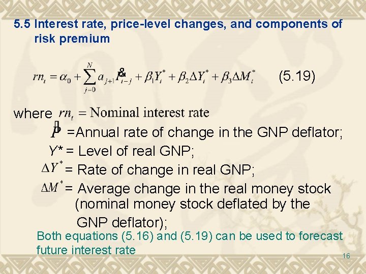
5. 5 Interest rate, price-level changes, and components of risk premium (5. 19) where =Annual rate of change in the GNP deflator; Y* = Level of real GNP; = Rate of change in real GNP; = Average change in the real money stock (nominal money stock deflated by the GNP deflator); Both equations (5. 16) and (5. 19) can be used to forecast future interest rate 16

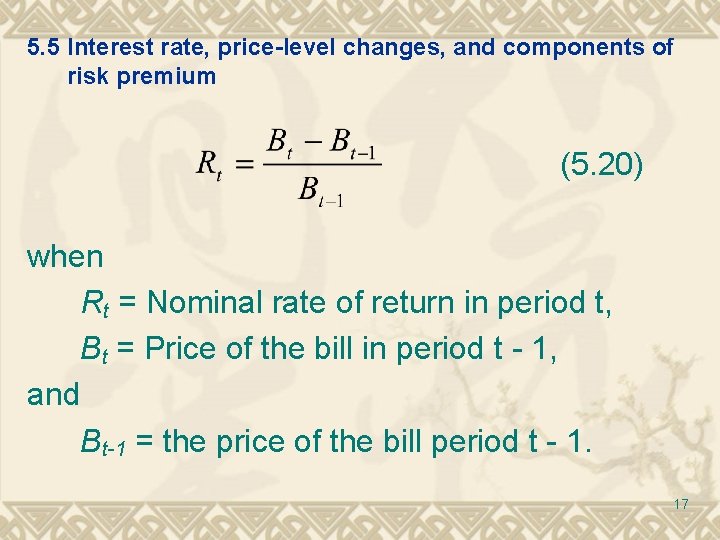
5. 5 Interest rate, price-level changes, and components of risk premium (5. 20) when Rt = Nominal rate of return in period t, Bt = Price of the bill in period t - 1, and Bt-1 = the price of the bill period t - 1. 17

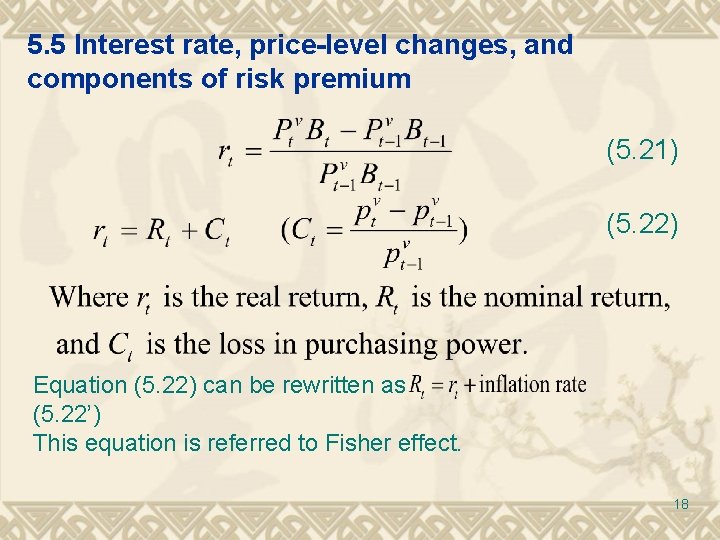
5. 5 Interest rate, price-level changes, and components of risk premium (5. 21) (5. 22) Equation (5. 22) can be rewritten as (5. 22’) This equation is referred to Fisher effect. 18

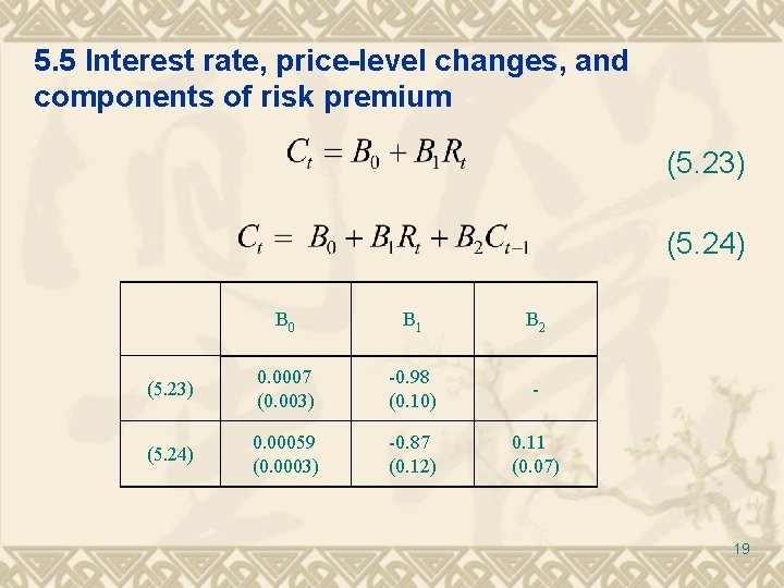
5. 5 Interest rate, price-level changes, and components of risk premium (5. 23) (5. 24) B 0 B 1 B 2 (5. 23) 0. 0007 (0. 003) -0. 98 (0. 10) - (5. 24) 0. 00059 (0. 0003) -0. 87 (0. 12) 0. 11 (0. 07) 19

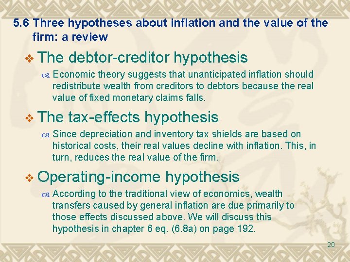
5. 6 Three hypotheses about inflation and the value of the firm: a review v The debtor-creditor hypothesis Economic theory suggests that unanticipated inflation should redistribute wealth from creditors to debtors because the real value of fixed monetary claims falls. v The tax-effects hypothesis Since depreciation and inventory tax shields are based on historical costs, their real values decline with inflation. This, in turn, reduces the real value of the firm. v Operating-income hypothesis According to the traditional view of economics, wealth transfers caused by general inflation are due primarily to those effects discussed above. We will discuss this hypothesis in chapter 6 eq. (6. 8 a) on page 192. 20

5. 7 Summary and concluding remarks In this chapter we have examined several concepts that will be of importance later. Determination of appropriate interest rates and risk premiums is very important in capital budgeting (Chapters 12 and 13), leasing (Chapter 14), and cost of capital determinations (Chapter 11). The mathematical concepts of arithmetic, geometric, and mixed means will also be important for estimating growth of dividends (Chapter 16) and financial planning and forecasting (Chapters 22 and 23). A basic understanding about the relationships between various types of risks (inflation, liquidity, and default) will be necessary for analyzing alternative risk premiums in financial analysis, planning, and forecasting. 21

Appendix 5 A. Compounding and discounting processes and their applications 5. A. 1 SINGLE-VALUE CASE a) Compound Future Sum (Terminal Value) b) Present Value v 5. A. 2 Annuity Case a) Compound Future Sum of An Annuity b) Present Value of An Annuity v 22

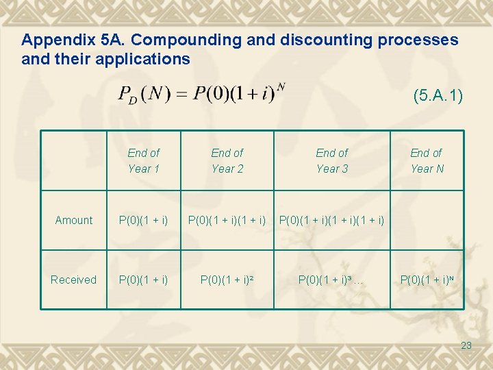
Appendix 5 A. Compounding and discounting processes and their applications (5. A. 1) End of Year 1 End of Year 2 End of Year 3 Amount P(0)(1 + i)(1 + i) Received P(0)(1 + i)2 P(0)(1 + i)3 End of Year N P(0)(1 + i)N 23

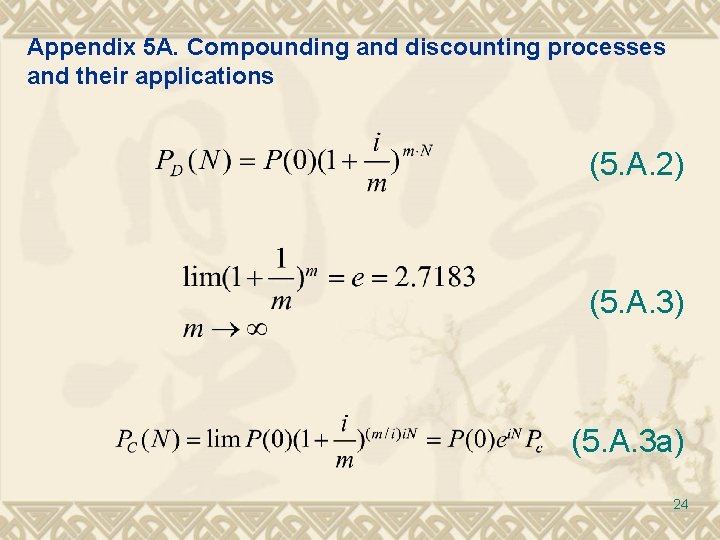
Appendix 5 A. Compounding and discounting processes and their applications (5. A. 2) (5. A. 3 a) 24

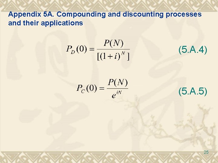
Appendix 5 A. Compounding and discounting processes and their applications (5. A. 4) (5. A. 5) 25

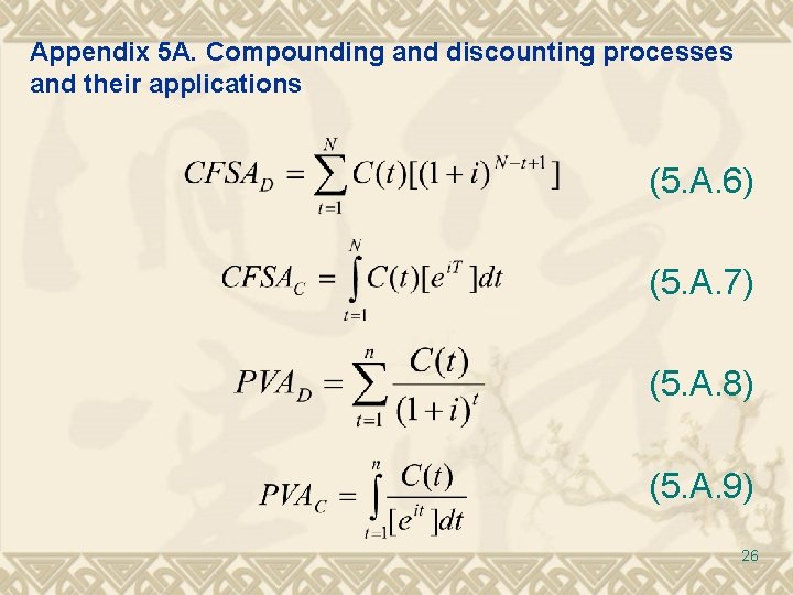
Appendix 5 A. Compounding and discounting processes and their applications (5. A. 6) (5. A. 7) (5. A. 8) (5. A. 9) 26

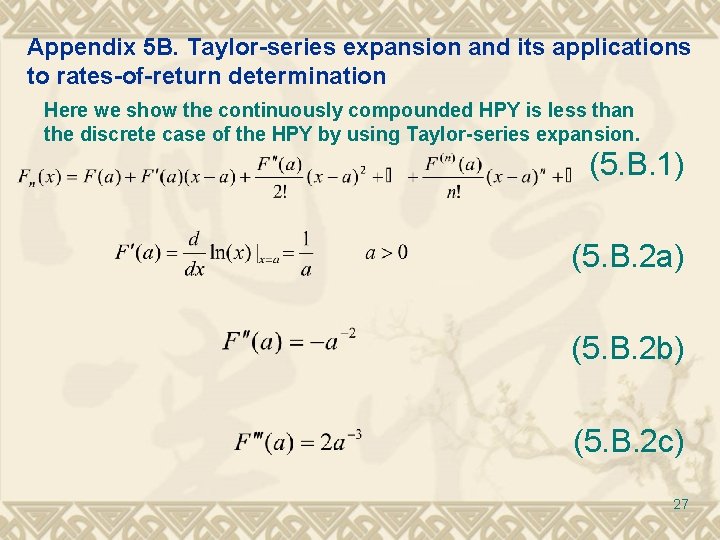
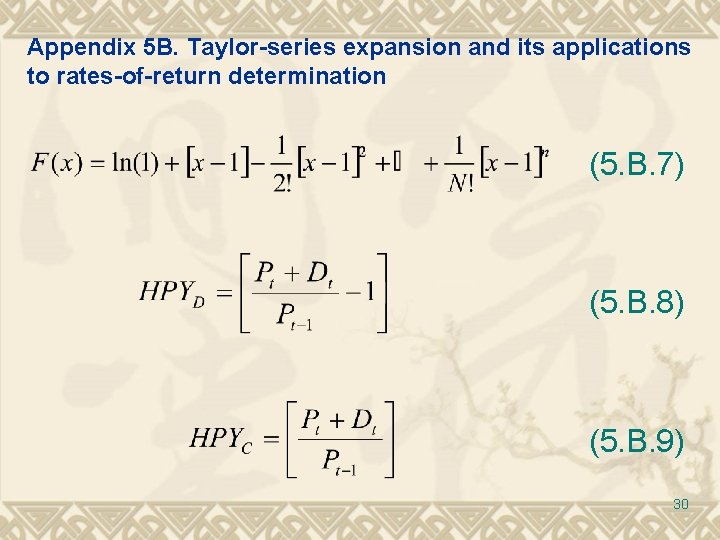
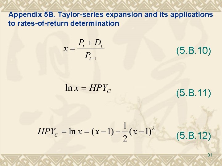
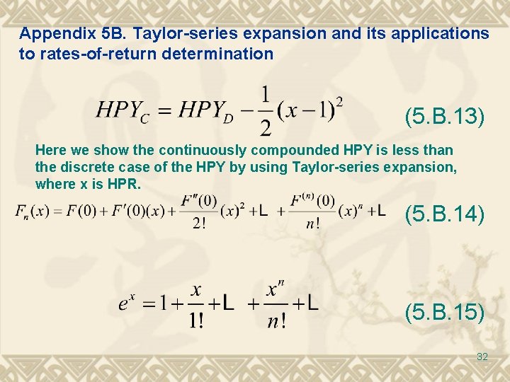
Appendix 5 B. Taylor-series expansion and its applications to rates-of-return determination Here we show the continuously compounded HPY is less than the discrete case of the HPY by using Taylor-series expansion. (5. B. 1) (5. B. 2 a) (5. B. 2 b) (5. B. 2 c) 27

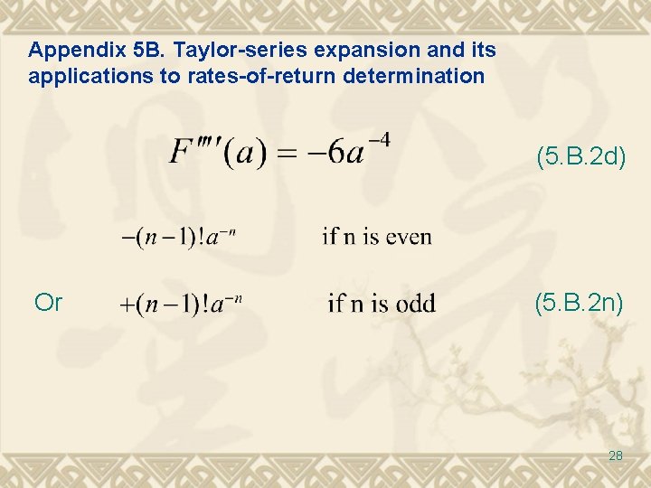
Appendix 5 B. Taylor-series expansion and its applications to rates-of-return determination (5. B. 2 d) Or (5. B. 2 n) 28

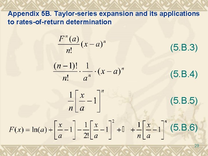
Appendix 5 B. Taylor-series expansion and its applications to rates-of-return determination (5. B. 3) (5. B. 4) (5. B. 5) (5. B. 6) 29

Appendix 5 B. Taylor-series expansion and its applications to rates-of-return determination (5. B. 7) (5. B. 8) (5. B. 9) 30

Appendix 5 B. Taylor-series expansion and its applications to rates-of-return determination (5. B. 10) (5. B. 11) (5. B. 12) 31

Appendix 5 B. Taylor-series expansion and its applications to rates-of-return determination (5. B. 13) Here we show the continuously compounded HPY is less than the discrete case of the HPY by using Taylor-series expansion, where x is HPR. (5. B. 14) (5. B. 15) 32

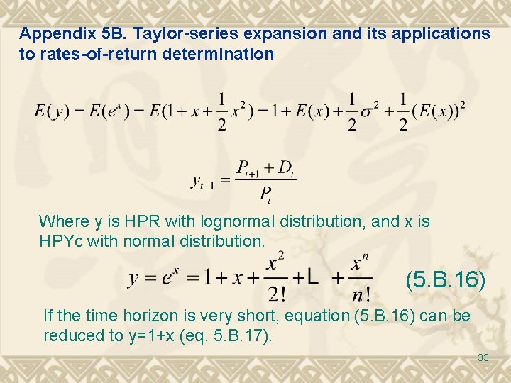
Appendix 5 B. Taylor-series expansion and its applications to rates-of-return determination Where y is HPR with lognormal distribution, and x is HPYc with normal distribution. (5. B. 16) If the time horizon is very short, equation (5. B. 16) can be reduced to y=1+x (eq. 5. B. 17). 33

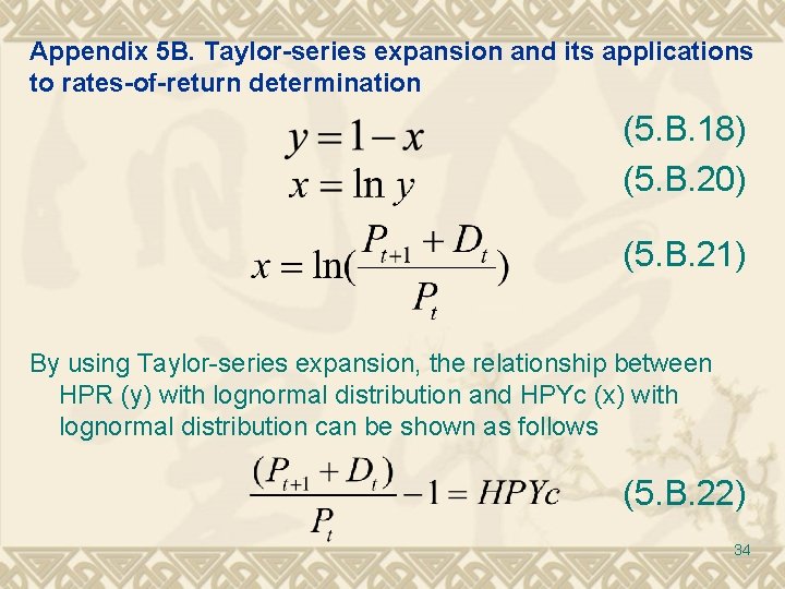
Appendix 5 B. Taylor-series expansion and its applications to rates-of-return determination (5. B. 18) (5. B. 20) (5. B. 21) By using Taylor-series expansion, the relationship between HPR (y) with lognormal distribution and HPYc (x) with lognormal distribution can be shown as follows (5. B. 22) 34

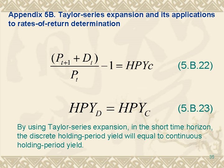
Appendix 5 B. Taylor-series expansion and its applications to rates-of-return determination (5. B. 22) (5. B. 23) By using Taylor-series expansion, in the short time horizon, the discrete holding-period yield will equal to continuous holding-period yield. 35