Chapter 12 Forecasting Russell and Taylor Operations and






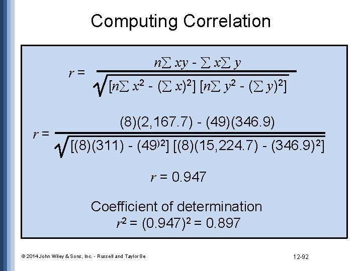
![Computing Correlation r= n xy - x y [n x 2 - ( x)2] Computing Correlation r= n xy - x y [n x 2 - ( x)2]](https://slidetodoc.com/presentation_image_h2/f3c76143dbcf0d85055a5395a1865c2e/image-91.jpg)
- Slides: 100

Chapter 12 Forecasting Russell and Taylor Operations and Supply Chain Management, 8 th Edition

© 2014 John Wiley & Sons, Inc. - Russell and Taylor 8 e 12 -2

© 2014 John Wiley & Sons, Inc. - Russell and Taylor 8 e 12 -3

© 2014 John Wiley & Sons, Inc. - Russell and Taylor 8 e 12 -4

© 2014 John Wiley & Sons, Inc. - Russell and Taylor 8 e 12 -5

Lecture Outline • Strategic Role of Forecasting in Supply Chain Management • Components of Forecasting Demand • Time Series Methods • Forecast Accuracy • Time Series Forecasting Using Excel • Regression Methods © 2014 John Wiley & Sons, Inc. - Russell and Taylor 8 e 12 -6

Learning Objectives • Discuss the strategic role of forecasting in supply chain management • Describe the forecasting process and identify the components of forecasting demand • Forecast demand using various time series models, including exponential smoothing, and trend and seasonal adjustments • Discuss and calculate various methods for evaluating forecast accuracy • Use Excel to create various forecast models • Develop forecasting models with linear and multiple regression analysis © 2014 John Wiley & Sons, Inc. - Russell and Taylor 8 e 12 -7

Forecasting • Predicting the future • Qualitative forecast methods • subjective • Quantitative forecast methods • based on mathematical formulas © 2014 John Wiley & Sons, Inc. - Russell and Taylor 8 e 12 -8

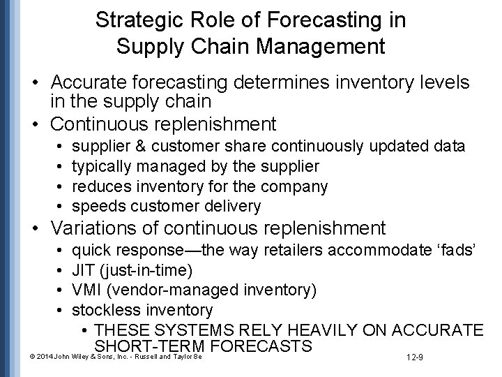
Strategic Role of Forecasting in Supply Chain Management • Accurate forecasting determines inventory levels in the supply chain • Continuous replenishment • • supplier & customer share continuously updated data typically managed by the supplier reduces inventory for the company speeds customer delivery • Variations of continuous replenishment • • quick response—the way retailers accommodate ‘fads’ JIT (just-in-time) VMI (vendor-managed inventory) stockless inventory • THESE SYSTEMS RELY HEAVILY ON ACCURATE SHORT-TERM FORECASTS © 2014 John Wiley & Sons, Inc. - Russell and Taylor 8 e 12 -9

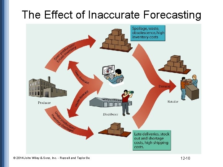
The Effect of Inaccurate Forecasting © 2014 John Wiley & Sons, Inc. - Russell and Taylor 8 e 12 -10

Forecasting • Quality Management • Accurately forecasting customer demand is a key to providing good quality service • Strategic Planning • Successful strategic planning requires accurate forecasts of future products and markets © 2014 John Wiley & Sons, Inc. - Russell and Taylor 8 e 12 -11

Components of Forecasting Demand • Time frame • Demand behavior • Causes of behavior © 2014 John Wiley & Sons, Inc. - Russell and Taylor 8 e 12 -12

Time Frame • Indicates how far into the future is forecast • Short-range forecast • typically encompasses the immediate future up to six months • Use for detailed scheduling of goods and services • Medium-range forecast • Six months to two years • 18 months is a typical medium-range forecast • Addresses aggregate planning—what HR, what inventory, what technology • Long-range forecast • usually encompasses a period of time longer than two years out to say 50 years with 5 years being a typical long-range forecast • Used to make capital investment decisions—what facilities located where, by when? © 2014 John Wiley & Sons, Inc. - Russell and Taylor 8 e 12 -13

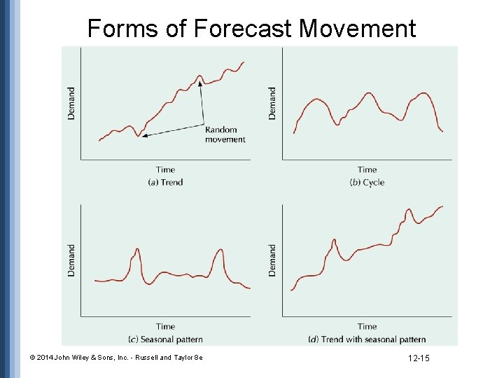
Demand Behavior • Trend • a gradual, long-term up or down movement of demand • Random variations • movements in demand that do not follow a pattern • Cycle • an up-and-down repetitive movement in demand • Seasonal pattern • an up-and-down repetitive movement in demand occurring periodically © 2014 John Wiley & Sons, Inc. - Russell and Taylor 8 e 12 -14

Forms of Forecast Movement © 2014 John Wiley & Sons, Inc. - Russell and Taylor 8 e 12 -15

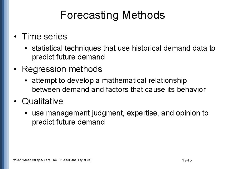
Forecasting Methods • Time series • statistical techniques that use historical demand data to predict future demand • Regression methods • attempt to develop a mathematical relationship between demand factors that cause its behavior • Qualitative • use management judgment, expertise, and opinion to predict future demand © 2014 John Wiley & Sons, Inc. - Russell and Taylor 8 e 12 -16

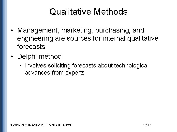
Qualitative Methods • Management, marketing, purchasing, and engineering are sources for internal qualitative forecasts • Delphi method • involves soliciting forecasts about technological advances from experts © 2014 John Wiley & Sons, Inc. - Russell and Taylor 8 e 12 -17

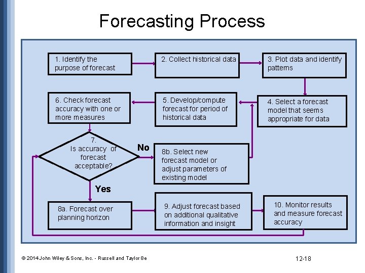
Forecasting Process 1. Identify the purpose of forecast 2. Collect historical data 3. Plot data and identify patterns 6. Check forecast accuracy with one or more measures 5. Develop/compute forecast for period of historical data 4. Select a forecast model that seems appropriate for data 7. Is accuracy of forecast acceptable? No 8 b. Select new forecast model or adjust parameters of existing model Yes 8 a. Forecast over planning horizon © 2014 John Wiley & Sons, Inc. - Russell and Taylor 8 e 9. Adjust forecast based on additional qualitative information and insight 10. Monitor results and measure forecast accuracy 12 -18

Data Mining • Process to analyze large amounts of data • A set of IT tools • Every day your transaction database is saved into the data warehouse • Identify patterns, trends and relationships among and between groups of customers, markets and products • This is driven by very low data storage costs • 1979: 15 megabyte hard-drive costs $1500 • About $100 per megabyte • 2017: 5 terabyte Seagate hard drive costs $133 • How many megabytes in a terabyte? 1, 000 • So one terabyte should cost $100, 000 in 1979 $ • 5 TB (terabytes) would be $500, 000 in 1979 $ © 2014 John Wiley & Sons, Inc. - Russell and Taylor 8 e 12 -19

Forecast when the price of gasoline will return to $3 a gallon : a DELPHI simulation • • Forecast when the price of gasoline will return to $3 a gallon • Write your answer on a piece of paper 11 -20

I’m a politician trying to sell you on the idea that as a country we should impose tariffs on imports • We run a $750 billion trade deficit with the rest of the world—that is exports minus imports • Our major trading partners are China, Mexico and Canada • In order to have balanced trade with these countries what should happen? • That would generate a lot of jobs in this country • It would increase our annual GDP from $18 T to nearly $19 T • Tell me why that may not be a good idea? © 2014 John Wiley & Sons, Inc. - Russell and Taylor 8 e 12 -21

Time Series • Time is often the independent variable in forecasting • Assumes that what has occurred in the past will continue to occur in the future • Relate the forecast to only one factor - time • Include • • naïve forecast moving average exponential smoothing linear trend line © 2014 John Wiley & Sons, Inc. - Russell and Taylor 8 e 12 -22

Moving Average • Naive forecast • demand in current period is used as next period’s forecast • Simple moving average • uses average demand for a fixed sequence of periods • good for stable demand with no pronounced behavioral patterns • Weighted moving average • weights are assigned to most recent data © 2014 John Wiley & Sons, Inc. - Russell and Taylor 8 e 12 -23

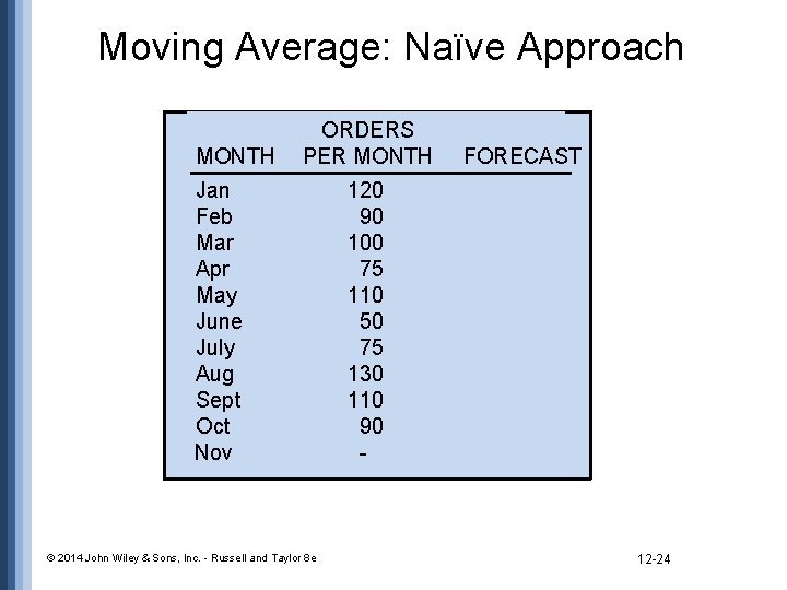
Moving Average: Naïve Approach MONTH ORDERS PER MONTH Jan Feb Mar Apr May June July Aug Sept Oct Nov © 2014 John Wiley & Sons, Inc. - Russell and Taylor 8 e FORECAST 120 90 100 75 110 50 75 130 110 90 - 12 -24

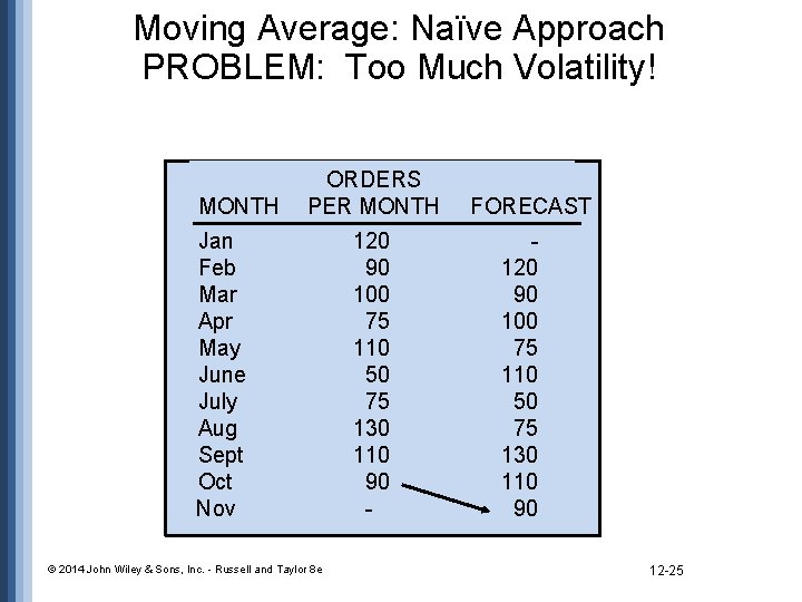
Moving Average: Naïve Approach PROBLEM: Too Much Volatility! MONTH ORDERS PER MONTH Jan Feb Mar Apr May June July Aug Sept Oct Nov © 2014 John Wiley & Sons, Inc. - Russell and Taylor 8 e 120 90 100 75 110 50 75 130 110 90 - FORECAST 120 90 100 75 110 50 75 130 110 90 12 -25

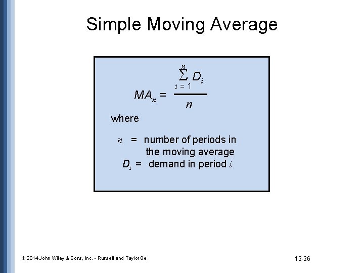
Simple Moving Average n Di MAn = i=1 n where n = number of periods in the moving average Di = demand in period i © 2014 John Wiley & Sons, Inc. - Russell and Taylor 8 e 12 -26

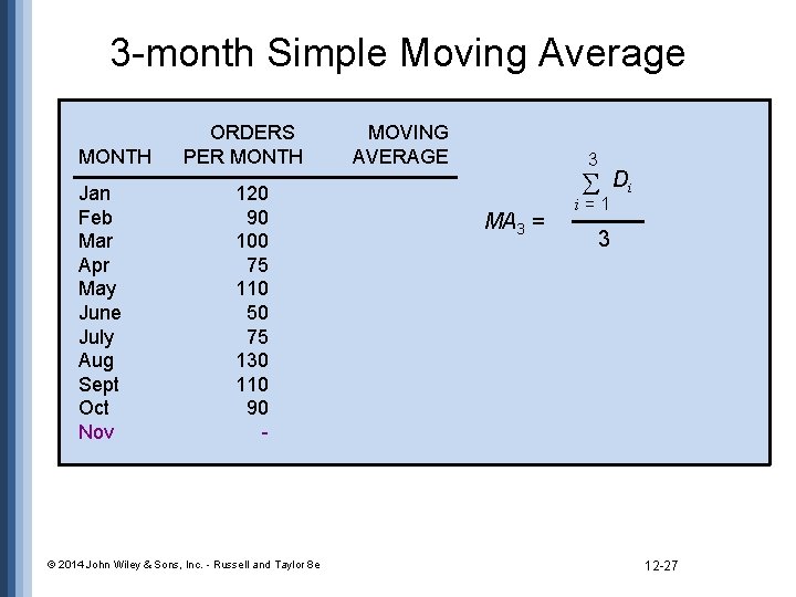
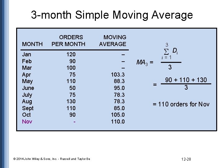
3 -month Simple Moving Average MONTH Jan Feb Mar Apr May June July Aug Sept Oct Nov ORDERS PER MONTH 120 90 100 75 110 50 75 130 110 90 - © 2014 John Wiley & Sons, Inc. - Russell and Taylor 8 e MOVING AVERAGE 3 MA 3 = i=1 Di 3 12 -27

3 -month Simple Moving Average MONTH Jan Feb Mar Apr May June July Aug Sept Oct Nov ORDERS PER MONTH 120 90 100 75 110 50 75 130 110 90 - © 2014 John Wiley & Sons, Inc. - Russell and Taylor 8 e MOVING AVERAGE – – – 103. 3 88. 3 95. 0 78. 3 85. 0 105. 0 110. 0 3 MA 3 = = i=1 Di 3 90 + 110 + 130 3 = 110 orders for Nov 12 -28

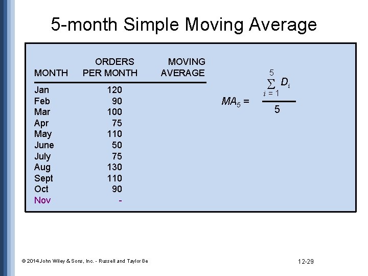
5 -month Simple Moving Average MONTH Jan Feb Mar Apr May June July Aug Sept Oct Nov ORDERS PER MONTH 120 90 100 75 110 50 75 130 110 90 - © 2014 John Wiley & Sons, Inc. - Russell and Taylor 8 e MOVING AVERAGE 5 MA 5 = i=1 Di 5 12 -29

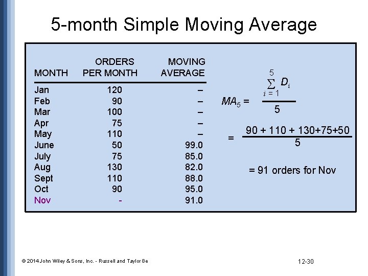
5 -month Simple Moving Average MONTH Jan Feb Mar Apr May June July Aug Sept Oct Nov ORDERS PER MONTH 120 90 100 75 110 50 75 130 110 90 - © 2014 John Wiley & Sons, Inc. - Russell and Taylor 8 e MOVING AVERAGE – – – 99. 0 85. 0 82. 0 88. 0 95. 0 91. 0 5 MA 5 = = i=1 Di 5 90 + 110 + 130+75+50 5 = 91 orders for Nov 12 -30

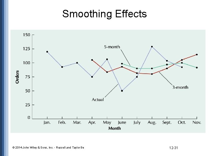
Smoothing Effects © 2014 John Wiley & Sons, Inc. - Russell and Taylor 8 e 12 -31

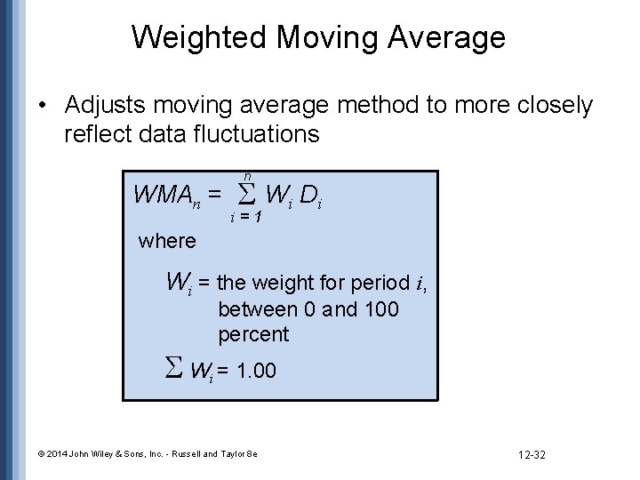
Weighted Moving Average • Adjusts moving average method to more closely reflect data fluctuations WMAn = n Wi Di i=1 where Wi = the weight for period i, between 0 and 100 percent Wi = 1. 00 © 2014 John Wiley & Sons, Inc. - Russell and Taylor 8 e 12 -32

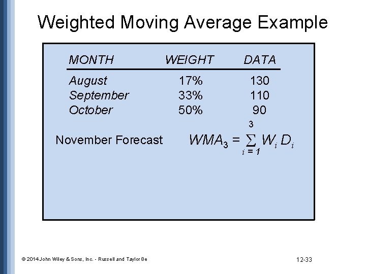
Weighted Moving Average Example MONTH August September October WEIGHT DATA 17% 33% 50% 130 110 90 3 November Forecast © 2014 John Wiley & Sons, Inc. - Russell and Taylor 8 e WMA 3 = Wi Di i=1 12 -33

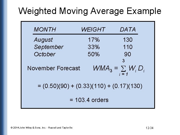
Weighted Moving Average Example MONTH August September October WEIGHT DATA 17% 33% 50% 130 110 90 3 November Forecast WMA 3 = Wi Di i=1 = (0. 50)(90) + (0. 33)(110) + (0. 17)(130) = 103. 4 orders © 2014 John Wiley & Sons, Inc. - Russell and Taylor 8 e 12 -34

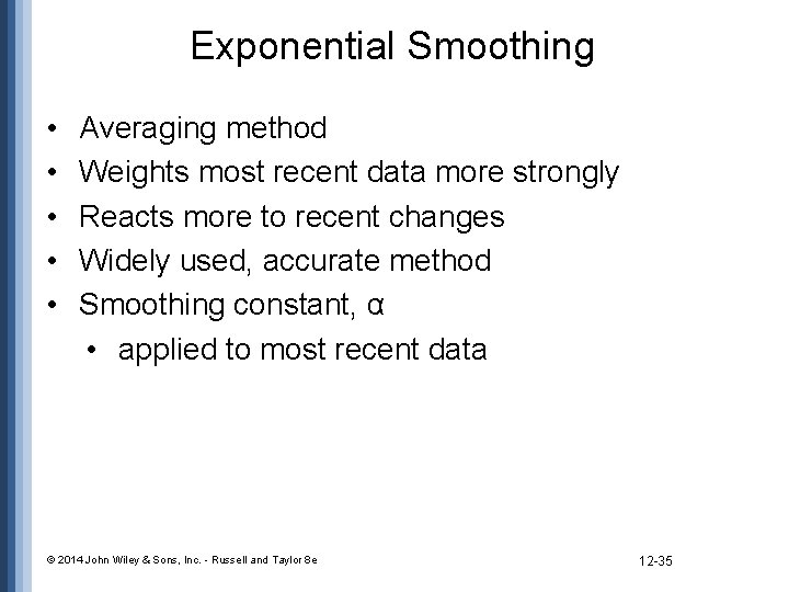
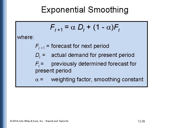
Exponential Smoothing • • • Averaging method Weights most recent data more strongly Reacts more to recent changes Widely used, accurate method Smoothing constant, α • applied to most recent data © 2014 John Wiley & Sons, Inc. - Russell and Taylor 8 e 12 -35

Exponential Smoothing Ft +1 = Dt + (1 - )Ft where: Ft +1 = forecast for next period Dt = actual demand for present period Ft = previously determined forecast for present period = weighting factor, smoothing constant © 2014 John Wiley & Sons, Inc. - Russell and Taylor 8 e 12 -36

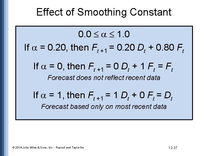
Effect of Smoothing Constant 0. 0 1. 0 If = 0. 20, then Ft +1 = 0. 20 Dt + 0. 80 Ft If = 0, then Ft +1 = 0 Dt + 1 Ft = Ft Forecast does not reflect recent data If = 1, then Ft +1 = 1 Dt + 0 Ft = Dt Forecast based only on most recent data © 2014 John Wiley & Sons, Inc. - Russell and Taylor 8 e 12 -37

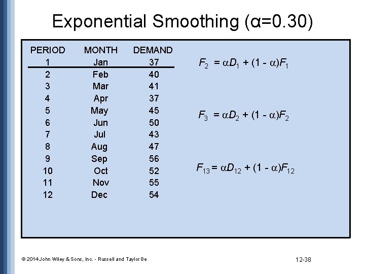
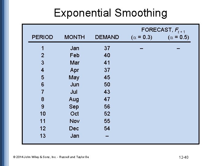
Exponential Smoothing (α=0. 30) PERIOD 1 2 3 4 5 6 7 8 9 10 11 12 MONTH Jan Feb Mar Apr May Jun Jul Aug Sep Oct Nov Dec DEMAND 37 40 41 37 45 50 43 47 56 52 55 54 © 2014 John Wiley & Sons, Inc. - Russell and Taylor 8 e F 2 = D 1 + (1 - )F 1 F 3 = D 2 + (1 - )F 2 F 13 = D 12 + (1 - )F 12 12 -38

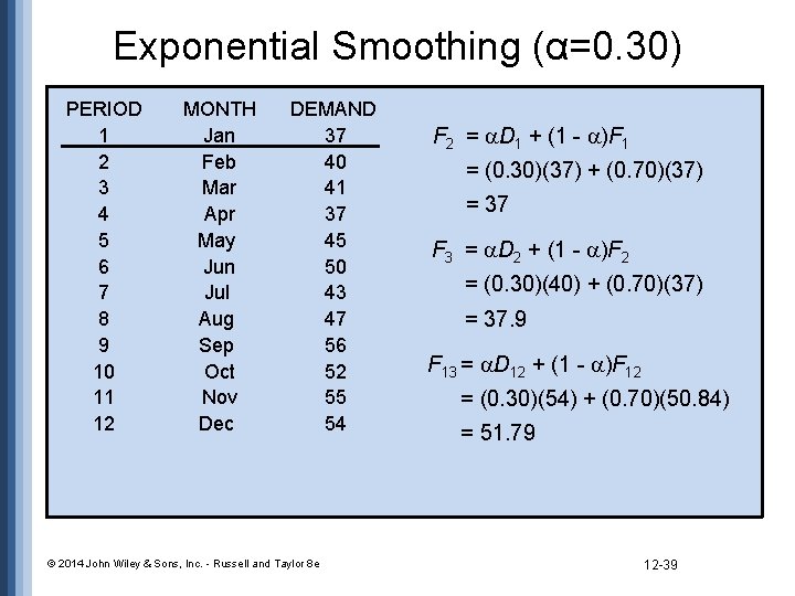
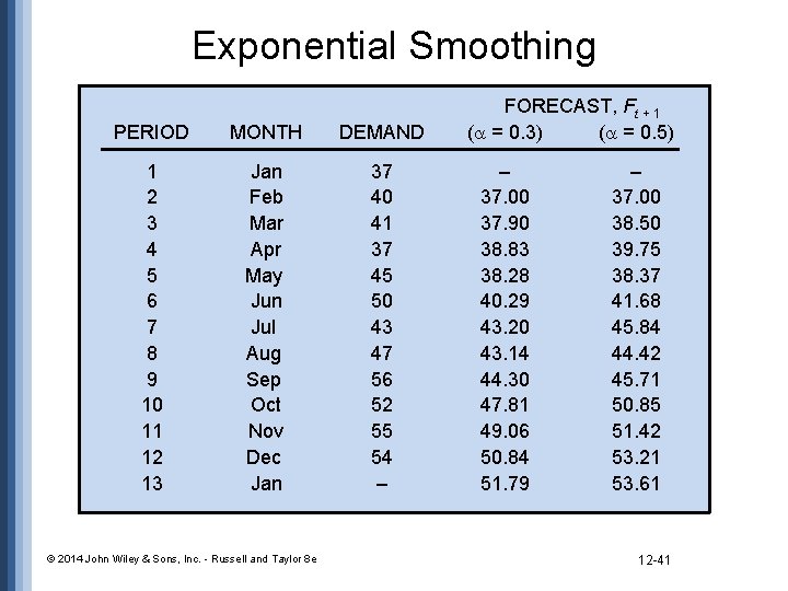
Exponential Smoothing (α=0. 30) PERIOD 1 2 3 4 5 6 7 8 9 10 11 12 MONTH Jan Feb Mar Apr May Jun Jul Aug Sep Oct Nov Dec DEMAND 37 40 41 37 45 50 43 47 56 52 55 54 © 2014 John Wiley & Sons, Inc. - Russell and Taylor 8 e F 2 = D 1 + (1 - )F 1 = (0. 30)(37) + (0. 70)(37) = 37 F 3 = D 2 + (1 - )F 2 = (0. 30)(40) + (0. 70)(37) = 37. 9 F 13 = D 12 + (1 - )F 12 = (0. 30)(54) + (0. 70)(50. 84) = 51. 79 12 -39

Exponential Smoothing PERIOD MONTH DEMAND 1 2 3 4 5 6 7 8 9 10 11 12 13 Jan Feb Mar Apr May Jun Jul Aug Sep Oct Nov Dec Jan 37 40 41 37 45 50 43 47 56 52 55 54 – © 2014 John Wiley & Sons, Inc. - Russell and Taylor 8 e FORECAST, Ft + 1 ( = 0. 3) ( = 0. 5) – – 12 -40

Exponential Smoothing PERIOD MONTH DEMAND 1 2 3 4 5 6 7 8 9 10 11 12 13 Jan Feb Mar Apr May Jun Jul Aug Sep Oct Nov Dec Jan 37 40 41 37 45 50 43 47 56 52 55 54 – © 2014 John Wiley & Sons, Inc. - Russell and Taylor 8 e FORECAST, Ft + 1 ( = 0. 3) ( = 0. 5) – 37. 00 37. 90 38. 83 38. 28 40. 29 43. 20 43. 14 44. 30 47. 81 49. 06 50. 84 51. 79 – 37. 00 38. 50 39. 75 38. 37 41. 68 45. 84 44. 42 45. 71 50. 85 51. 42 53. 21 53. 61 12 -41

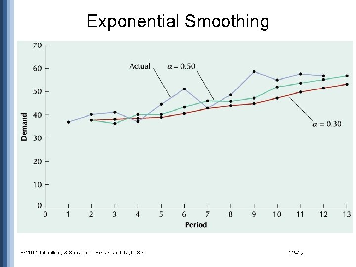
Exponential Smoothing © 2014 John Wiley & Sons, Inc. - Russell and Taylor 8 e 12 -42

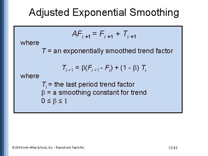
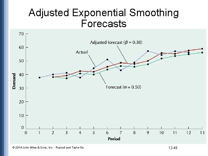
Adjusted Exponential Smoothing where AFt +1 = Ft +1 + Tt +1 T = an exponentially smoothed trend factor where Tt +1 = (Ft +1 - Ft) + (1 - ) Tt Tt = the last period trend factor = a smoothing constant for trend 0 ≤ ≤ 1 © 2014 John Wiley & Sons, Inc. - Russell and Taylor 8 e 12 -43

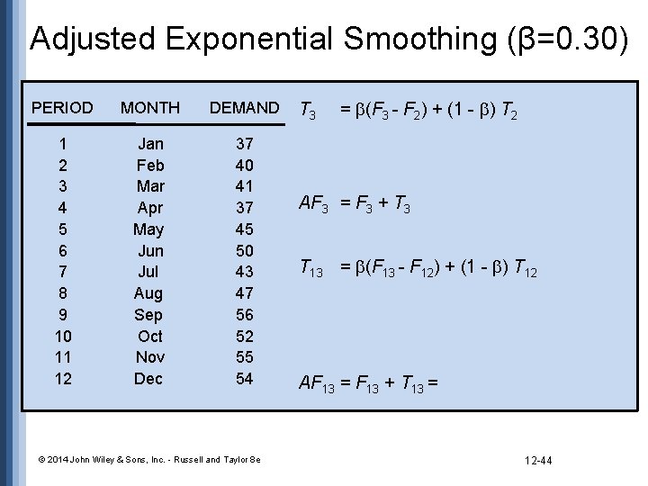
Adjusted Exponential Smoothing (β=0. 30) PERIOD MONTH DEMAND 1 2 3 4 5 6 7 8 9 10 11 12 Jan Feb Mar Apr May Jun Jul Aug Sep Oct Nov Dec 37 40 41 37 45 50 43 47 56 52 55 54 © 2014 John Wiley & Sons, Inc. - Russell and Taylor 8 e T 3 = (F 3 - F 2) + (1 - ) T 2 AF 3 = F 3 + T 3 T 13 = (F 13 - F 12) + (1 - ) T 12 AF 13 = F 13 + T 13 = 12 -44

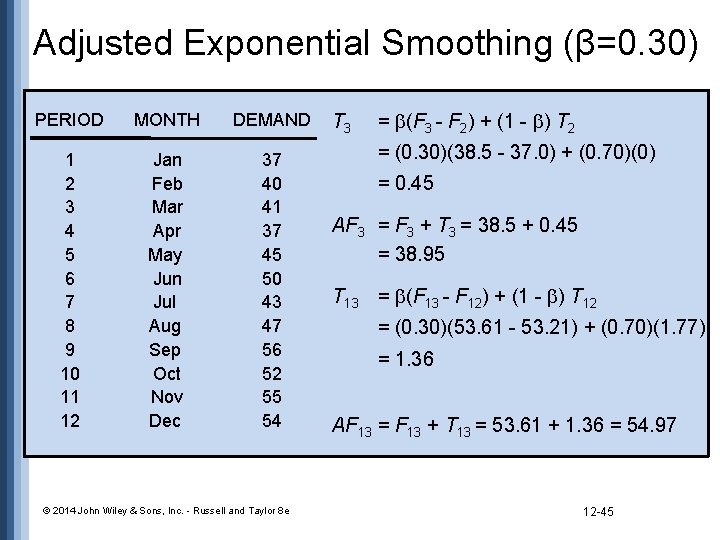
Adjusted Exponential Smoothing (β=0. 30) PERIOD MONTH DEMAND 1 2 3 4 5 6 7 8 9 10 11 12 Jan Feb Mar Apr May Jun Jul Aug Sep Oct Nov Dec 37 40 41 37 45 50 43 47 56 52 55 54 © 2014 John Wiley & Sons, Inc. - Russell and Taylor 8 e T 3 = (F 3 - F 2) + (1 - ) T 2 = (0. 30)(38. 5 - 37. 0) + (0. 70)(0) = 0. 45 AF 3 = F 3 + T 3 = 38. 5 + 0. 45 = 38. 95 T 13 = (F 13 - F 12) + (1 - ) T 12 = (0. 30)(53. 61 - 53. 21) + (0. 70)(1. 77) = 1. 36 AF 13 = F 13 + T 13 = 53. 61 + 1. 36 = 54. 97 12 -45

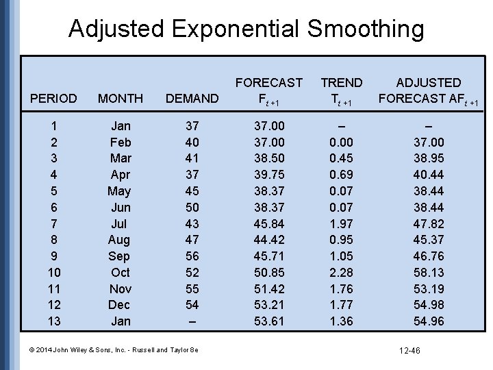
Adjusted Exponential Smoothing PERIOD MONTH DEMAND FORECAST Ft +1 1 2 3 4 5 6 7 8 9 10 11 12 13 Jan Feb Mar Apr May Jun Jul Aug Sep Oct Nov Dec Jan 37 40 41 37 45 50 43 47 56 52 55 54 – 37. 00 38. 50 39. 75 38. 37 45. 84 44. 42 45. 71 50. 85 51. 42 53. 21 53. 61 © 2014 John Wiley & Sons, Inc. - Russell and Taylor 8 e TREND Tt +1 ADJUSTED FORECAST AFt +1 – 0. 00 0. 45 0. 69 0. 07 1. 97 0. 95 1. 05 2. 28 1. 76 1. 77 1. 36 – 37. 00 38. 95 40. 44 38. 44 47. 82 45. 37 46. 76 58. 13 53. 19 54. 98 54. 96 12 -46

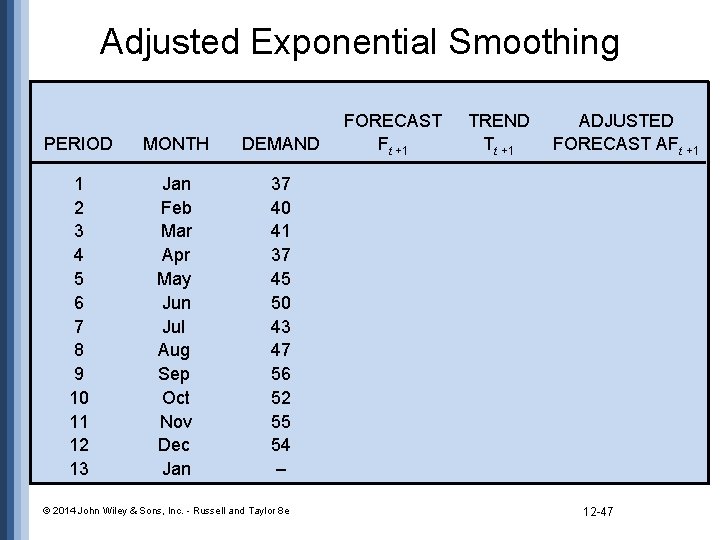
Adjusted Exponential Smoothing PERIOD MONTH DEMAND 1 2 3 4 5 6 7 8 9 10 11 12 13 Jan Feb Mar Apr May Jun Jul Aug Sep Oct Nov Dec Jan 37 40 41 37 45 50 43 47 56 52 55 54 – © 2014 John Wiley & Sons, Inc. - Russell and Taylor 8 e FORECAST Ft +1 TREND Tt +1 ADJUSTED FORECAST AFt +1 12 -47

Adjusted Exponential Smoothing Forecasts © 2014 John Wiley & Sons, Inc. - Russell and Taylor 8 e 12 -48

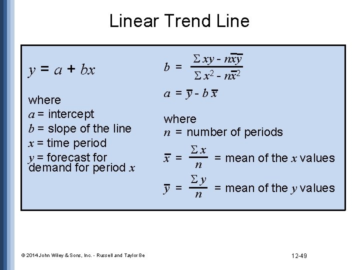
Linear Trend Line y = a + bx where a = intercept b = slope of the line x = time period y = forecast for demand for period x © 2014 John Wiley & Sons, Inc. - Russell and Taylor 8 e xy - nxy b = x 2 - nx 2 a = y-bx where n = number of periods x x = n = mean of the x values y y = n = mean of the y values 12 -49

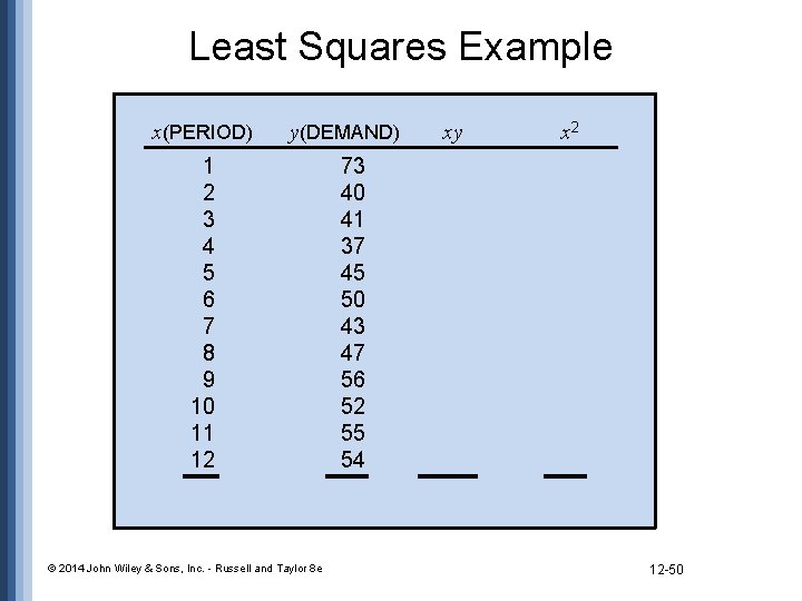
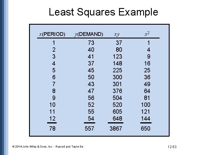
Least Squares Example x(PERIOD) y(DEMAND) 1 2 3 4 5 6 7 8 9 10 11 12 © 2014 John Wiley & Sons, Inc. - Russell and Taylor 8 e xy x 2 73 40 41 37 45 50 43 47 56 52 55 54 12 -50

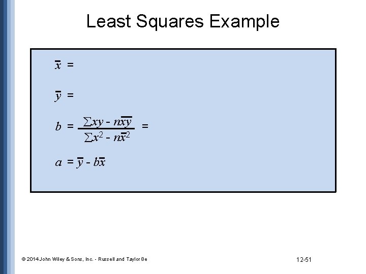
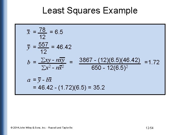
Least Squares Example x = y = b = xy - nxy = x 2 - nx 2 a = y - bx © 2014 John Wiley & Sons, Inc. - Russell and Taylor 8 e 12 -51

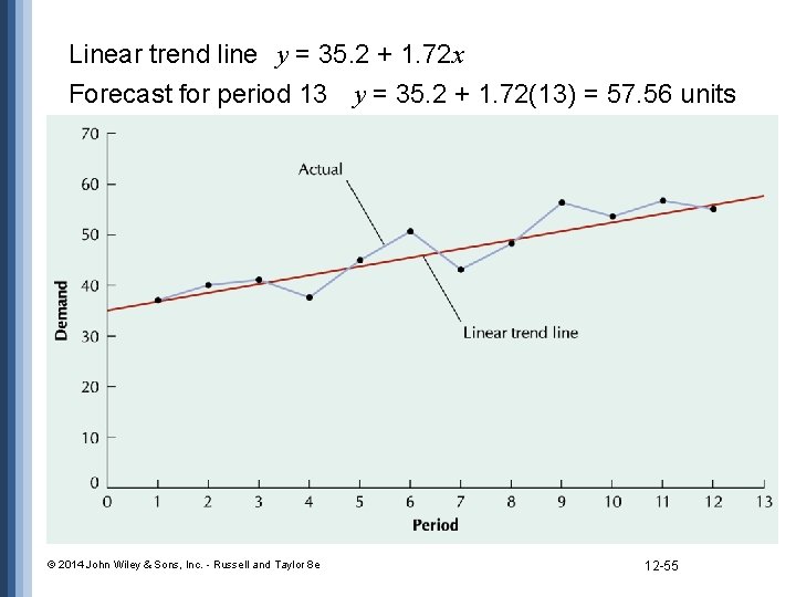
Linear trend line y = 35. 2 + 1. 72 x Forecast for period 13 y = 35. 2 + 1. 72(13) = 57. 56 units © 2014 John Wiley & Sons, Inc. - Russell and Taylor 8 e 12 -52

Least Squares Example x(PERIOD) y(DEMAND) xy x 2 1 2 3 4 5 6 7 8 9 10 11 12 73 40 41 37 45 50 43 47 56 52 55 54 37 80 123 148 225 300 301 376 504 520 605 648 1 4 9 16 25 36 49 64 81 100 121 144 78 557 3867 650 © 2014 John Wiley & Sons, Inc. - Russell and Taylor 8 e 12 -53

Least Squares Example x = 78 = 6. 5 12 y = 557 = 46. 42 12 b = xy - nxy = x 2 - nx 2 3867 - (12)(6. 5)(46. 42) =1. 72 650 - 12(6. 5)2 a = y - bx = 46. 42 - (1. 72)(6. 5) = 35. 2 © 2014 John Wiley & Sons, Inc. - Russell and Taylor 8 e 12 -54

Linear trend line y = 35. 2 + 1. 72 x Forecast for period 13 y = 35. 2 + 1. 72(13) = 57. 56 units © 2014 John Wiley & Sons, Inc. - Russell and Taylor 8 e 12 -55

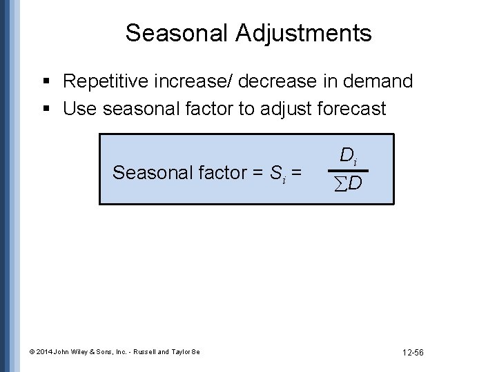
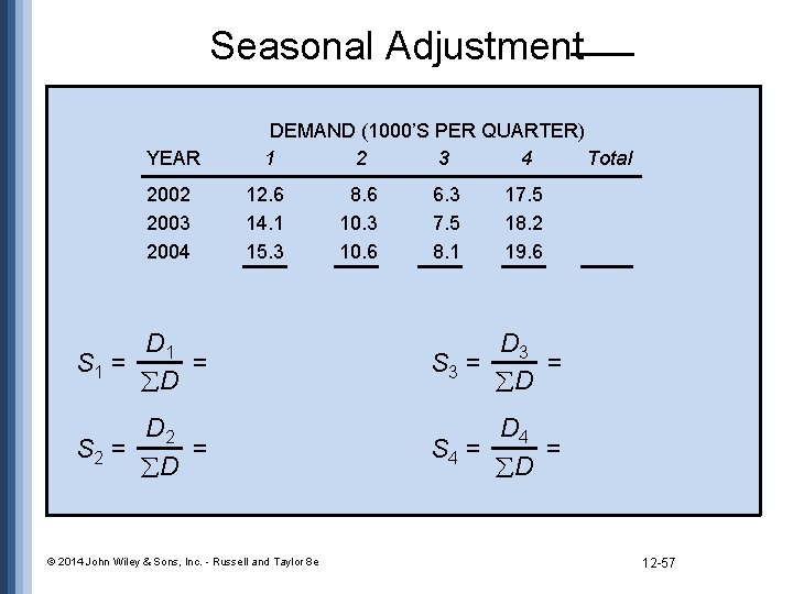
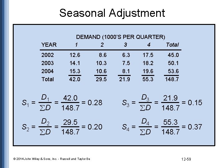
Seasonal Adjustments § Repetitive increase/ decrease in demand § Use seasonal factor to adjust forecast Seasonal factor = Si = © 2014 John Wiley & Sons, Inc. - Russell and Taylor 8 e Di D 12 -56

Seasonal Adjustment YEAR 2002 2003 2004 DEMAND (1000’S PER QUARTER) 1 2 3 4 Total 12. 6 14. 1 15. 3 8. 6 10. 3 10. 6 6. 3 7. 5 8. 1 17. 5 18. 2 19. 6 D 1 S 1 = = D D 3 S 3 = = D D 2 S 2 = = D D 4 S 4 = = D © 2014 John Wiley & Sons, Inc. - Russell and Taylor 8 e 12 -57

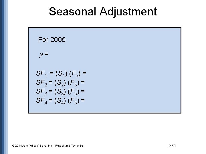
Seasonal Adjustment For 2005 y= SF 1 = (S 1) (F 5) = SF 2 = (S 2) (F 5) = SF 3 = (S 3) (F 5) = SF 4 = (S 4) (F 5) = © 2014 John Wiley & Sons, Inc. - Russell and Taylor 8 e 12 -58

Seasonal Adjustment YEAR 2002 2003 2004 Total DEMAND (1000’S PER QUARTER) 1 2 3 4 Total 12. 6 14. 1 15. 3 42. 0 8. 6 10. 3 10. 6 29. 5 6. 3 7. 5 8. 1 21. 9 17. 5 18. 2 19. 6 55. 3 45. 0 50. 1 53. 6 148. 7 D 1 42. 0 S 1 = = = 0. 28 D 148. 7 D 3 21. 9 S 3 = = = 0. 15 D 148. 7 D 2 29. 5 S 2 = = = 0. 20 D 148. 7 D 4 55. 3 S 4 = = = 0. 37 D 148. 7 © 2014 John Wiley & Sons, Inc. - Russell and Taylor 8 e 12 -59

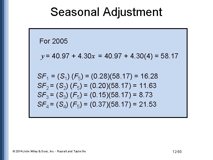
Seasonal Adjustment For 2005 y = 40. 97 + 4. 30 x = 40. 97 + 4. 30(4) = 58. 17 SF 1 = (S 1) (F 5) = (0. 28)(58. 17) = 16. 28 SF 2 = (S 2) (F 5) = (0. 20)(58. 17) = 11. 63 SF 3 = (S 3) (F 5) = (0. 15)(58. 17) = 8. 73 SF 4 = (S 4) (F 5) = (0. 37)(58. 17) = 21. 53 © 2014 John Wiley & Sons, Inc. - Russell and Taylor 8 e 12 -60

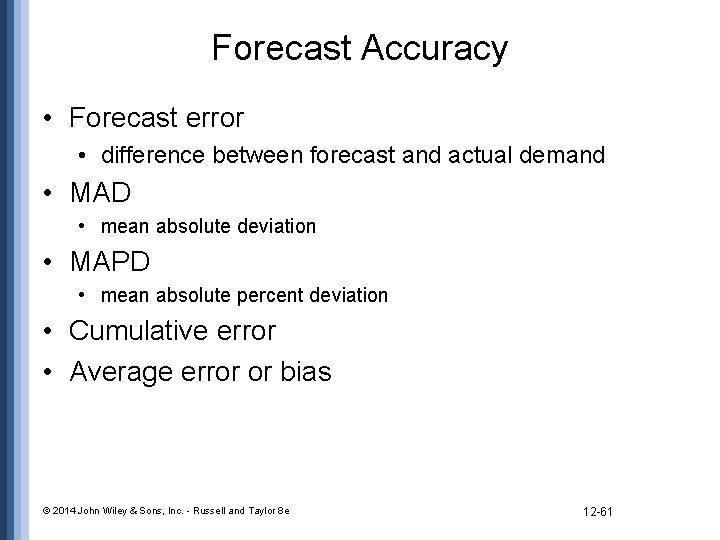
Forecast Accuracy • Forecast error • difference between forecast and actual demand • MAD • mean absolute deviation • MAPD • mean absolute percent deviation • Cumulative error • Average error or bias © 2014 John Wiley & Sons, Inc. - Russell and Taylor 8 e 12 -61

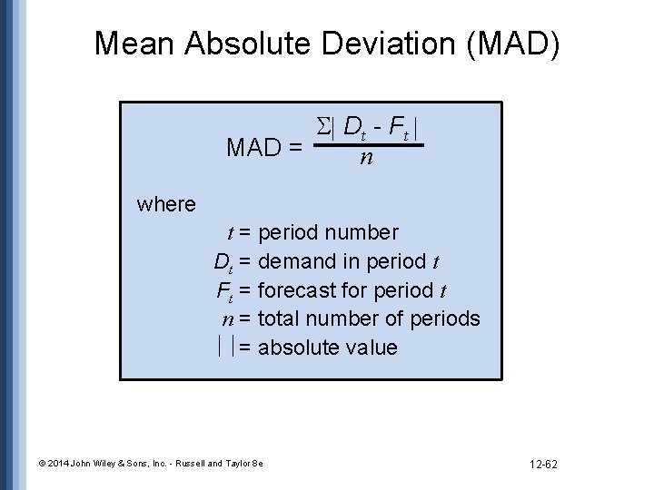
Mean Absolute Deviation (MAD) Dt - F t MAD = n where t = period number Dt = demand in period t Ft = forecast for period t n = total number of periods = absolute value © 2014 John Wiley & Sons, Inc. - Russell and Taylor 8 e 12 -62

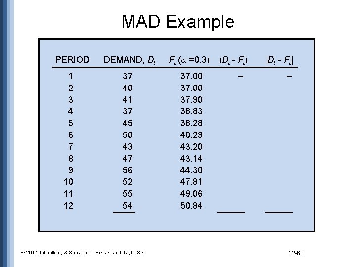
MAD Example PERIOD 1 2 3 4 5 6 7 8 9 10 11 12 DEMAND, Dt Ft ( =0. 3) 37 40 41 37 45 50 43 47 56 52 55 54 37. 00 37. 90 38. 83 38. 28 40. 29 43. 20 43. 14 44. 30 47. 81 49. 06 50. 84 © 2014 John Wiley & Sons, Inc. - Russell and Taylor 8 e (Dt - Ft) – |Dt - Ft| – 12 -63

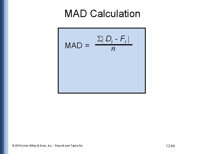
MAD Calculation Dt - F t MAD = n © 2014 John Wiley & Sons, Inc. - Russell and Taylor 8 e 12 -64

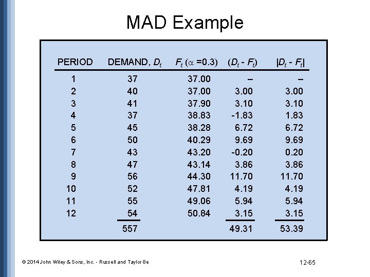
MAD Example PERIOD 1 2 3 4 5 6 7 8 9 10 11 12 DEMAND, Dt Ft ( =0. 3) (Dt - Ft) |Dt - Ft| 37 40 41 37 45 50 43 47 56 52 55 54 37. 00 37. 90 38. 83 38. 28 40. 29 43. 20 43. 14 44. 30 47. 81 49. 06 50. 84 – 3. 00 3. 10 -1. 83 6. 72 9. 69 -0. 20 3. 86 11. 70 4. 19 5. 94 3. 15 – 3. 00 3. 10 1. 83 6. 72 9. 69 0. 20 3. 86 11. 70 4. 19 5. 94 3. 15 49. 31 53. 39 557 © 2014 John Wiley & Sons, Inc. - Russell and Taylor 8 e 12 -65

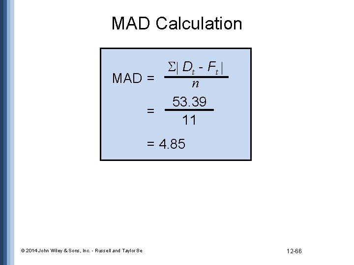
MAD Calculation Dt - F t MAD = n 53. 39 = 11 = 4. 85 © 2014 John Wiley & Sons, Inc. - Russell and Taylor 8 e 12 -66

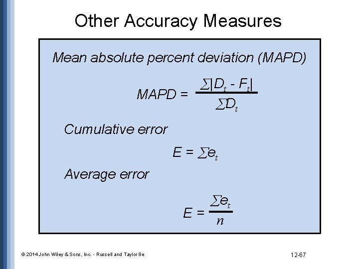
Other Accuracy Measures Mean absolute percent deviation (MAPD) |Dt - Ft| MAPD = Dt Cumulative error E = et Average error et E= n © 2014 John Wiley & Sons, Inc. - Russell and Taylor 8 e 12 -67

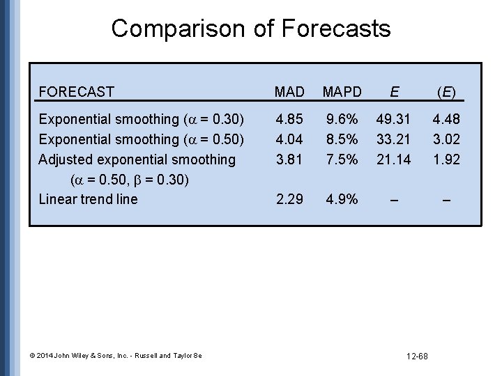
Comparison of Forecasts FORECAST MAD MAPD E (E) Exponential smoothing ( = 0. 30) Exponential smoothing ( = 0. 50) Adjusted exponential smoothing ( = 0. 50, = 0. 30) Linear trend line 4. 85 4. 04 3. 81 9. 6% 8. 5% 7. 5% 49. 31 33. 21 21. 14 4. 48 3. 02 1. 92 2. 29 4. 9% – – © 2014 John Wiley & Sons, Inc. - Russell and Taylor 8 e 12 -68

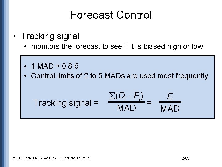
Forecast Control • Tracking signal • monitors the forecast to see if it is biased high or low • 1 MAD ≈ 0. 8 б • Control limits of 2 to 5 MADs are used most frequently Tracking signal = © 2014 John Wiley & Sons, Inc. - Russell and Taylor 8 e (Dt - Ft) E = MAD 12 -69

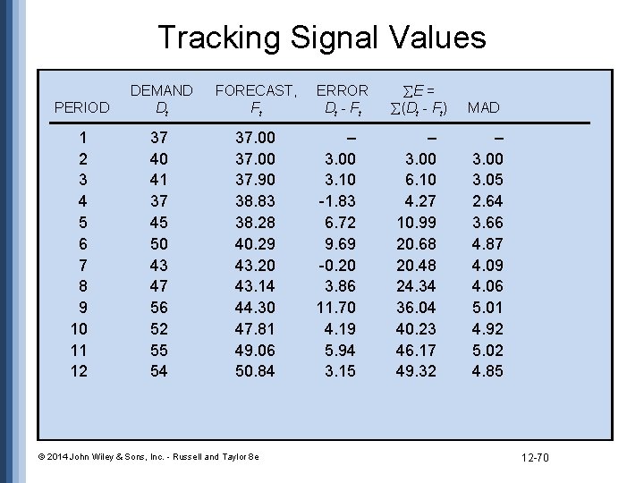
Tracking Signal Values PERIOD DEMAND Dt FORECAST, Ft 1 2 3 4 5 6 7 8 9 10 11 12 37 40 41 37 45 50 43 47 56 52 55 54 37. 00 37. 90 38. 83 38. 28 40. 29 43. 20 43. 14 44. 30 47. 81 49. 06 50. 84 © 2014 John Wiley & Sons, Inc. - Russell and Taylor 8 e ERROR Dt - F t – 3. 00 3. 10 -1. 83 6. 72 9. 69 -0. 20 3. 86 11. 70 4. 19 5. 94 3. 15 E = (Dt - Ft) MAD – 3. 00 6. 10 4. 27 10. 99 20. 68 20. 48 24. 34 36. 04 40. 23 46. 17 49. 32 – 3. 00 3. 05 2. 64 3. 66 4. 87 4. 09 4. 06 5. 01 4. 92 5. 02 4. 85 12 -70

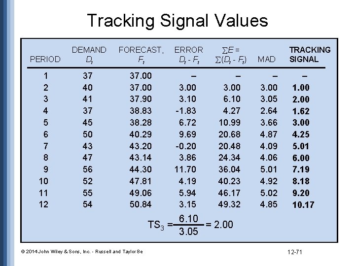
Tracking Signal Values PERIOD DEMAND Dt FORECAST, Ft 1 2 3 4 5 6 7 8 9 10 11 12 37 40 41 37 45 50 43 47 56 52 55 54 37. 00 37. 90 38. 83 38. 28 40. 29 43. 20 43. 14 44. 30 47. 81 49. 06 50. 84 TS 3 = © 2014 John Wiley & Sons, Inc. - Russell and Taylor 8 e ERROR Dt - F t – 3. 00 3. 10 -1. 83 6. 72 9. 69 -0. 20 3. 86 11. 70 4. 19 5. 94 3. 15 E = (Dt - Ft) MAD – 3. 00 6. 10 4. 27 10. 99 20. 68 20. 48 24. 34 36. 04 40. 23 46. 17 49. 32 – 3. 00 3. 05 2. 64 3. 66 4. 87 4. 09 4. 06 5. 01 4. 92 5. 02 4. 85 TRACKING SIGNAL – 1. 00 2. 00 1. 62 3. 00 4. 25 5. 01 6. 00 7. 19 8. 18 9. 20 10. 17 6. 10 = 2. 00 3. 05 12 -71

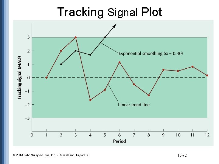
Tracking Signal Plot © 2014 John Wiley & Sons, Inc. - Russell and Taylor 8 e 12 -72

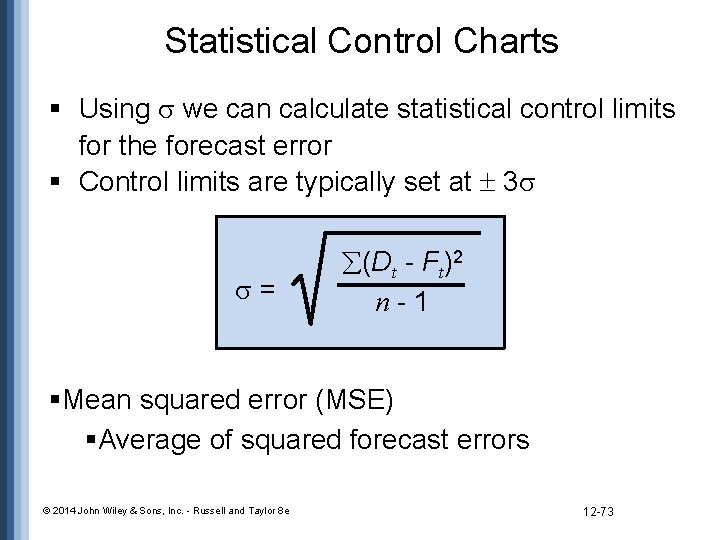
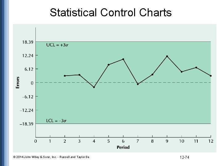
Statistical Control Charts § Using we can calculate statistical control limits for the forecast error § Control limits are typically set at 3 = (Dt - Ft)2 n-1 §Mean squared error (MSE) §Average of squared forecast errors © 2014 John Wiley & Sons, Inc. - Russell and Taylor 8 e 12 -73

Statistical Control Charts © 2014 John Wiley & Sons, Inc. - Russell and Taylor 8 e 12 -74

Time Series Forecasting Using Excel • Excel can be used to develop forecasts: • • Moving average Exponential smoothing Adjusted exponential smoothing Linear trend line © 2014 John Wiley & Sons, Inc. - Russell and Taylor 8 e 12 -75

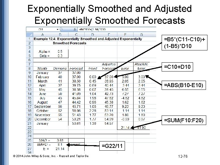
Exponentially Smoothed and Adjusted Exponentially Smoothed Forecasts =B 5*(C 11 -C 10)+ (1 -B 5)*D 10 =C 10+D 10 =ABS(B 10 -E 10) =SUM(F 10: F 20) =G 22/11 © 2014 John Wiley & Sons, Inc. - Russell and Taylor 8 e 12 -76

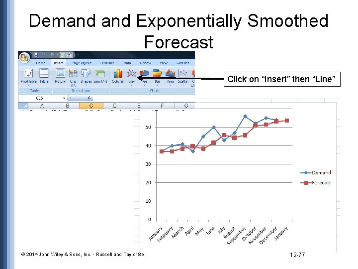
Demand Exponentially Smoothed Forecast Click on “Insert” then “Line” © 2014 John Wiley & Sons, Inc. - Russell and Taylor 8 e 12 -77

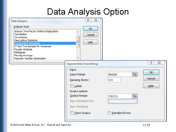
Data Analysis Option © 2014 John Wiley & Sons, Inc. - Russell and Taylor 8 e 12 -78

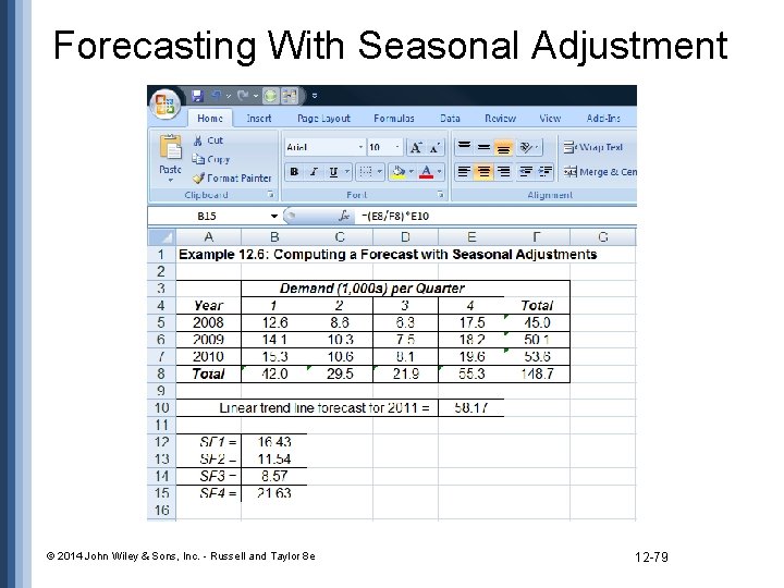
Forecasting With Seasonal Adjustment © 2014 John Wiley & Sons, Inc. - Russell and Taylor 8 e 12 -79

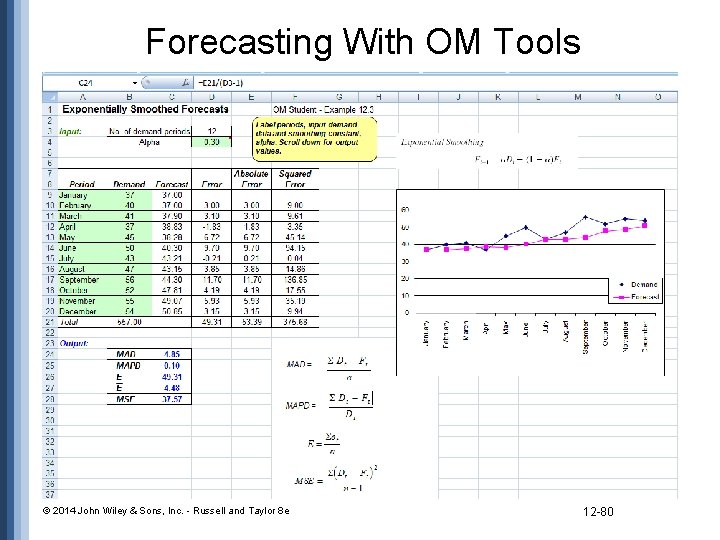
Forecasting With OM Tools © 2014 John Wiley & Sons, Inc. - Russell and Taylor 8 e 12 -80

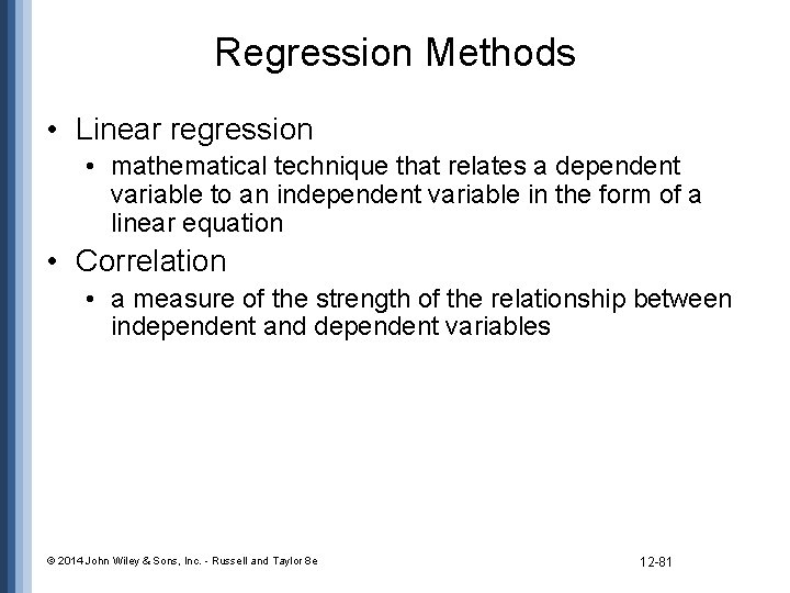
Regression Methods • Linear regression • mathematical technique that relates a dependent variable to an independent variable in the form of a linear equation • Correlation • a measure of the strength of the relationship between independent and dependent variables © 2014 John Wiley & Sons, Inc. - Russell and Taylor 8 e 12 -81

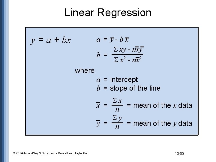
Linear Regression y = a + bx a = y-bx xy - nxy b = x 2 - nx 2 where a = intercept b = slope of the line x x = = mean of the x data n y y = n = mean of the y data © 2014 John Wiley & Sons, Inc. - Russell and Taylor 8 e 12 -82

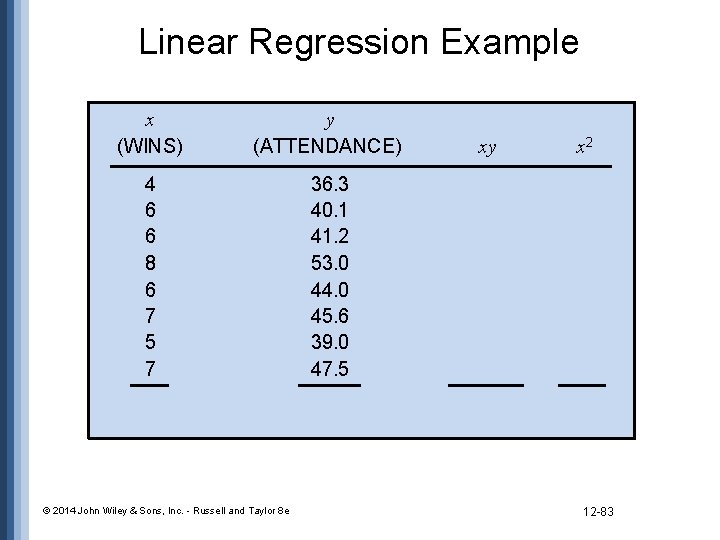
Linear Regression Example x (WINS) y (ATTENDANCE) 4 6 6 8 6 7 5 7 36. 3 40. 1 41. 2 53. 0 44. 0 45. 6 39. 0 47. 5 © 2014 John Wiley & Sons, Inc. - Russell and Taylor 8 e xy x 2 12 -83

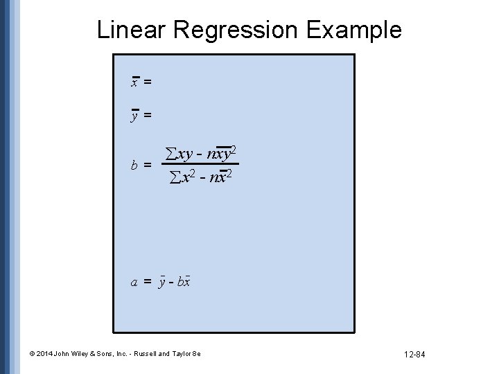
Linear Regression Example x= y= xy - nxy 2 b= x 2 - nx 2 a = y - bx © 2014 John Wiley & Sons, Inc. - Russell and Taylor 8 e 12 -84

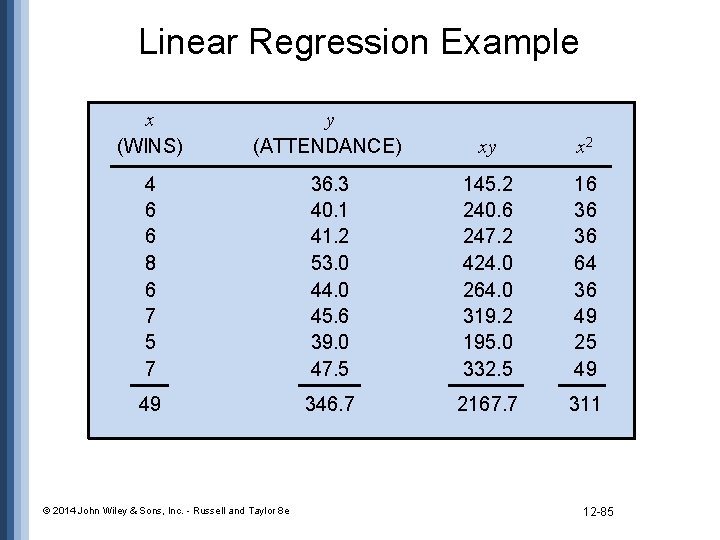
Linear Regression Example x (WINS) y (ATTENDANCE) xy x 2 4 6 6 8 6 7 5 7 36. 3 40. 1 41. 2 53. 0 44. 0 45. 6 39. 0 47. 5 145. 2 240. 6 247. 2 424. 0 264. 0 319. 2 195. 0 332. 5 16 36 36 64 36 49 25 49 49 346. 7 2167. 7 311 © 2014 John Wiley & Sons, Inc. - Russell and Taylor 8 e 12 -85

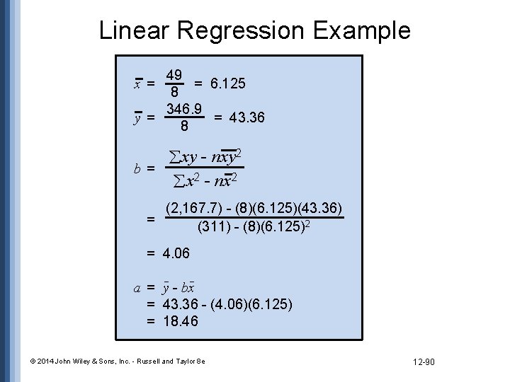
Linear Regression Example 49 = 6. 125 8 346. 9 y= = 43. 36 8 x= xy - nxy 2 b= x 2 - nx 2 (2, 167. 7) - (8)(6. 125)(43. 36) = (311) - (8)(6. 125)2 = 4. 06 a = y - bx = 43. 36 - (4. 06)(6. 125) = 18. 46 © 2014 John Wiley & Sons, Inc. - Russell and Taylor 8 e 12 -86

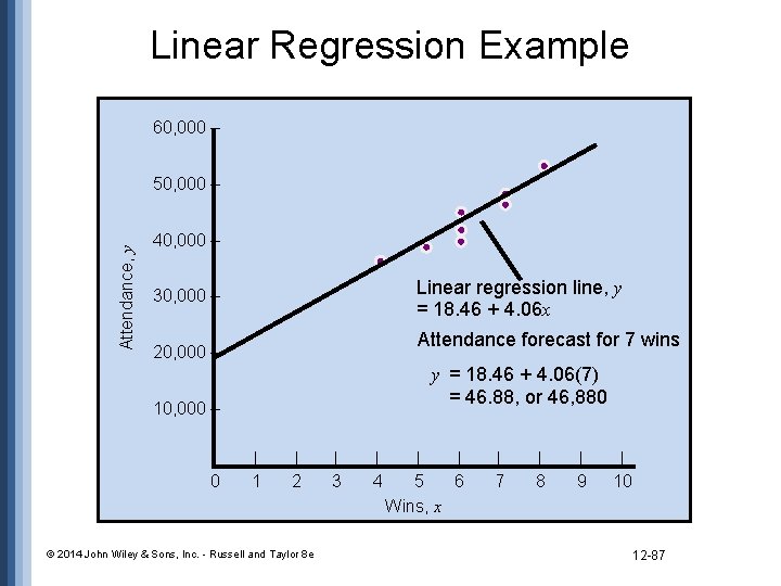
Linear Regression Example 60, 000 – Attendance, y 50, 000 – 40, 000 – Linear regression line, y = 18. 46 + 4. 06 x 30, 000 – Attendance forecast for 7 wins 20, 000 – y = 18. 46 + 4. 06(7) = 46. 88, or 46, 880 10, 000 – | 0 | 1 | 2 © 2014 John Wiley & Sons, Inc. - Russell and Taylor 8 e | 3 | 4 | | 5 6 Wins, x | 7 | 8 | 9 | 10 12 -87

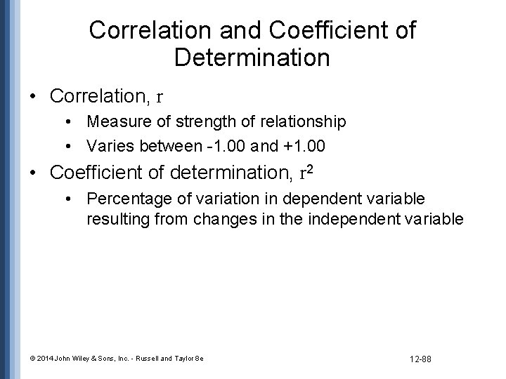
Correlation and Coefficient of Determination • Correlation, r • Measure of strength of relationship • Varies between -1. 00 and +1. 00 • Coefficient of determination, r 2 • Percentage of variation in dependent variable resulting from changes in the independent variable © 2014 John Wiley & Sons, Inc. - Russell and Taylor 8 e 12 -88

Linear Regression Example x (WINS) y (ATTENDANCE) xy x 2 4 6 6 8 6 7 5 7 36. 3 40. 1 41. 2 53. 0 44. 0 45. 6 39. 0 47. 5 145. 2 240. 6 247. 2 424. 0 264. 0 319. 2 195. 0 332. 5 16 36 36 64 36 49 25 49 49 346. 7 2167. 7 311 © 2014 John Wiley & Sons, Inc. - Russell and Taylor 8 e 12 -89

Linear Regression Example 49 = 6. 125 8 346. 9 y= = 43. 36 8 x= xy - nxy 2 b= x 2 - nx 2 (2, 167. 7) - (8)(6. 125)(43. 36) = (311) - (8)(6. 125)2 = 4. 06 a = y - bx = 43. 36 - (4. 06)(6. 125) = 18. 46 © 2014 John Wiley & Sons, Inc. - Russell and Taylor 8 e 12 -90
![Computing Correlation r n xy x y n x 2 x2 Computing Correlation r= n xy - x y [n x 2 - ( x)2]](https://slidetodoc.com/presentation_image_h2/f3c76143dbcf0d85055a5395a1865c2e/image-91.jpg)
Computing Correlation r= n xy - x y [n x 2 - ( x)2] [n y 2 - ( y)2] © 2014 John Wiley & Sons, Inc. - Russell and Taylor 8 e 12 -91

Computing Correlation r= r= n xy - x y [n x 2 - ( x)2] [n y 2 - ( y)2] (8)(2, 167. 7) - (49)(346. 9) [(8)(311) - (49)2] [(8)(15, 224. 7) - (346. 9)2] r = 0. 947 Coefficient of determination r 2 = (0. 947)2 = 0. 897 © 2014 John Wiley & Sons, Inc. - Russell and Taylor 8 e 12 -92

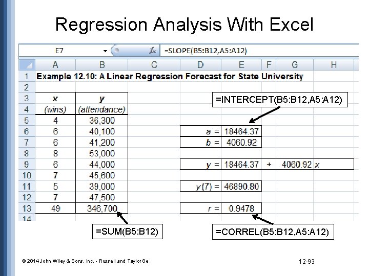
Regression Analysis With Excel =INTERCEPT(B 5: B 12, A 5: A 12) =SUM(B 5: B 12) © 2014 John Wiley & Sons, Inc. - Russell and Taylor 8 e =CORREL(B 5: B 12, A 5: A 12) 12 -93

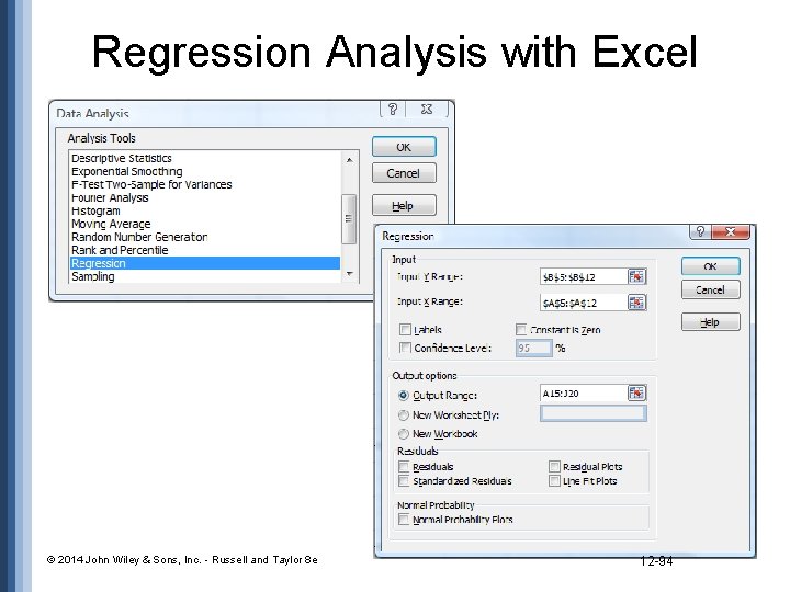
Regression Analysis with Excel © 2014 John Wiley & Sons, Inc. - Russell and Taylor 8 e 12 -94

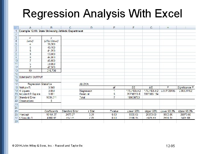
Regression Analysis With Excel © 2014 John Wiley & Sons, Inc. - Russell and Taylor 8 e 12 -95

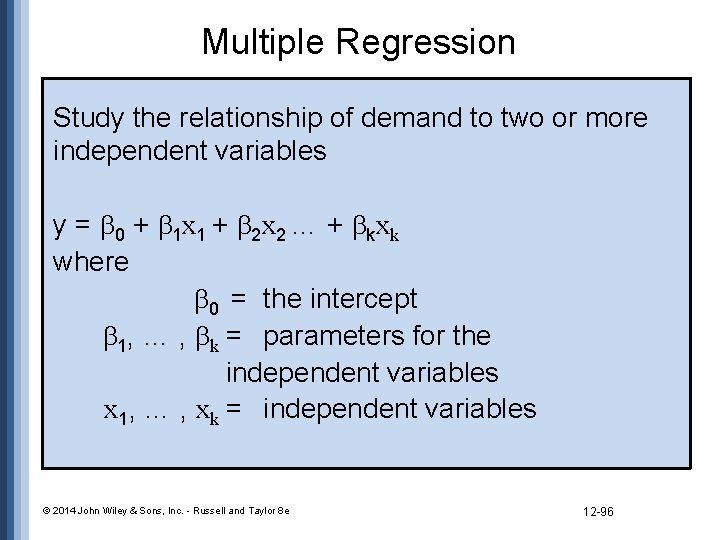
Multiple Regression Study the relationship of demand to two or more independent variables y = 0 + 1 x 1 + 2 x 2 … + kxk where 0 = the intercept 1, … , k = parameters for the independent variables x 1, … , xk = independent variables © 2014 John Wiley & Sons, Inc. - Russell and Taylor 8 e 12 -96

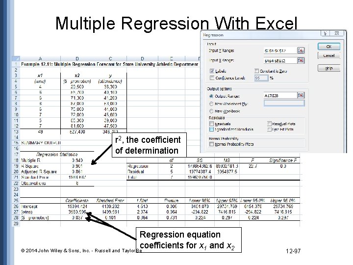
Multiple Regression With Excel r 2, the coefficient of determination Regression equation coefficients for x 1 and x 2 © 2014 John Wiley & Sons, Inc. - Russell and Taylor 8 e 12 -97

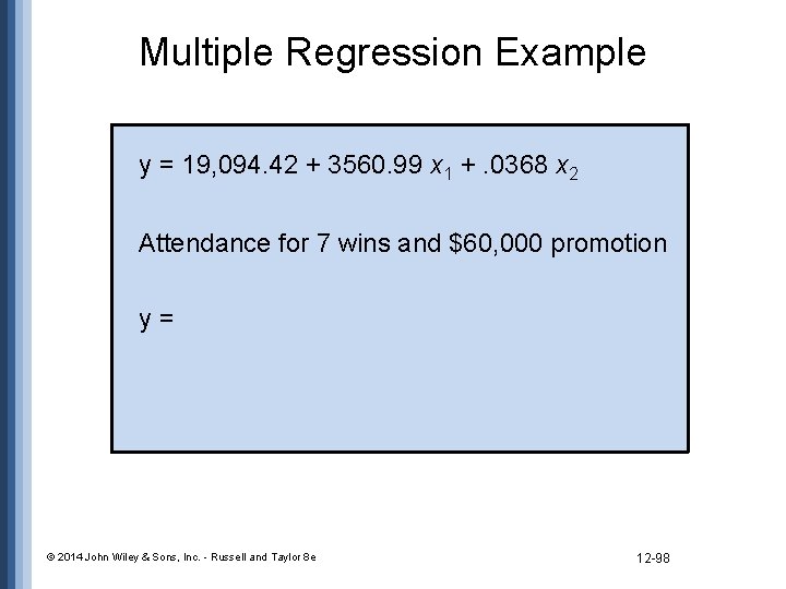
Multiple Regression Example y = 19, 094. 42 + 3560. 99 x 1 +. 0368 x 2 Attendance for 7 wins and $60, 000 promotion y= © 2014 John Wiley & Sons, Inc. - Russell and Taylor 8 e 12 -98

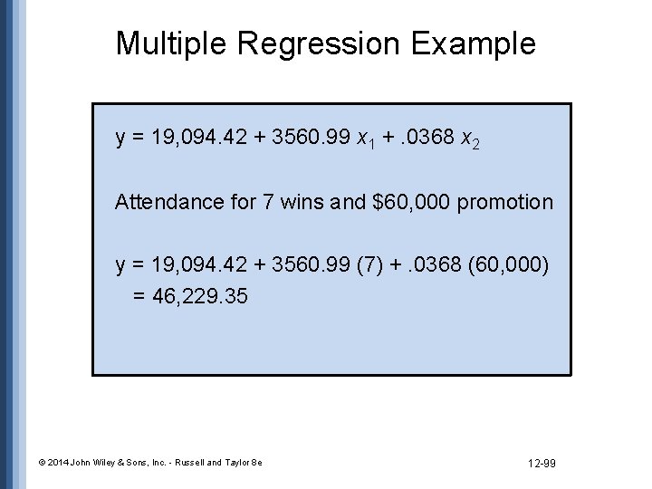
Multiple Regression Example y = 19, 094. 42 + 3560. 99 x 1 +. 0368 x 2 Attendance for 7 wins and $60, 000 promotion y = 19, 094. 42 + 3560. 99 (7) +. 0368 (60, 000) = 46, 229. 35 © 2014 John Wiley & Sons, Inc. - Russell and Taylor 8 e 12 -99

Copyright 2014 John Wiley & Sons, Inc. All rights reserved. Reproduction or translation of this work beyond that permitted in section 117 of the 1976 United States Copyright Act without express permission of the copyright owner is unlawful. Request for further information should be addressed to the Permission Department, John Wiley & Sons, Inc. The purchaser may make back-up copies for his/her own use only and not for distribution or resale. The Publisher assumes no responsibility for errors, omissions, or damages caused by the use of these programs or from the use of the information herein. © 2014 John Wiley & Sons, Inc. - Russell and Taylor 8 e 12 -100