Data Structures Algorithms Lecture 10 Elementary Graph Algorithms

Data Structures & Algorithms Lecture 10: Elementary Graph Algorithms

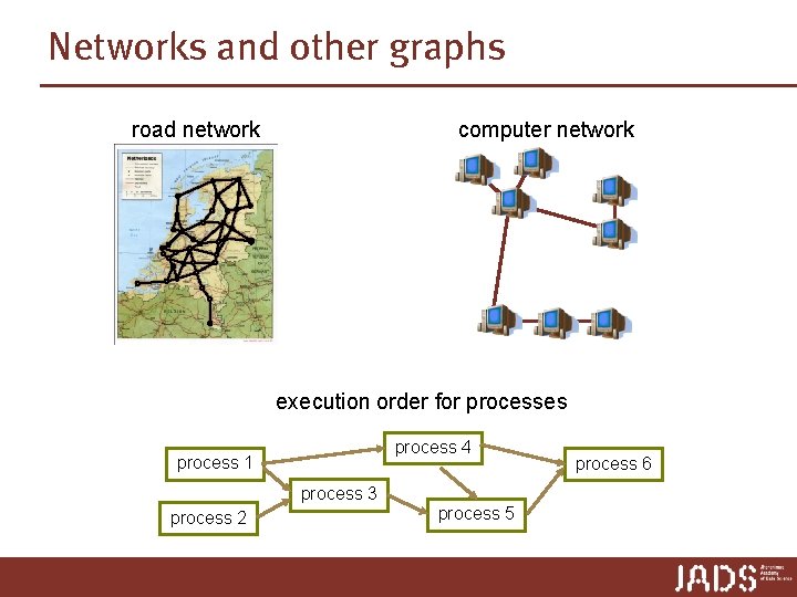
Networks and other graphs road network computer network execution order for processes process 4 process 1 process 3 process 2 process 5 process 6

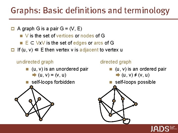
Graphs: Basic definitions and terminology p A graph G is a pair G = (V, E) n V is the set of vertices or nodes of G n E ⊂ Vx. V is the set of edges or arcs of G p If (u, v) ∈ E then vertex v is adjacent to vertex u undirected graph n (u, v) is an unordered pair ➨ (u, v) = (v, u) n self-loops forbidden directed graph n (u, v) is an ordered pair ➨ (u, v) ≠ (v, u) n self-loops possible

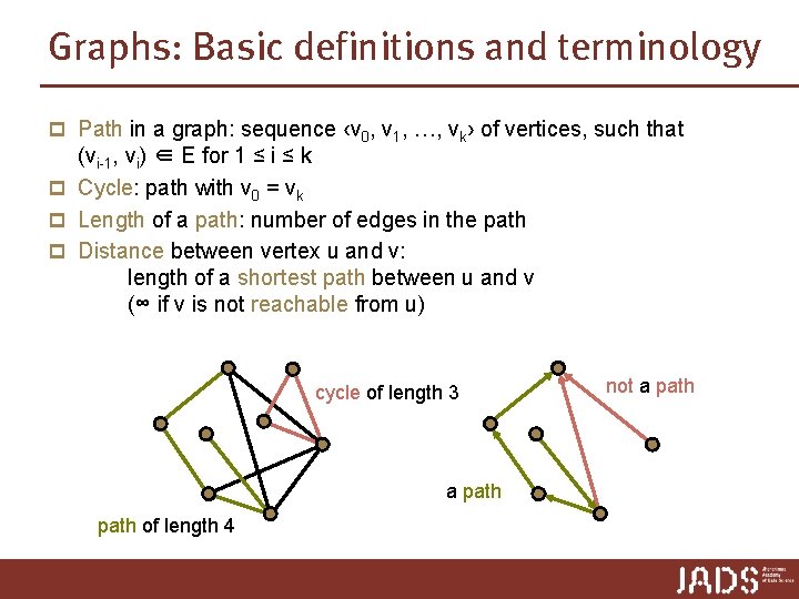
Graphs: Basic definitions and terminology p Path in a graph: sequence ‹v 0, v 1, …, vk› of vertices, such that (vi-1, vi) ∈ E for 1 ≤ i ≤ k p Cycle: path with v 0 = vk p Length of a path: number of edges in the path p Distance between vertex u and v: length of a shortest path between u and v (∞ if v is not reachable from u) cycle of length 3 a path of length 4 not a path

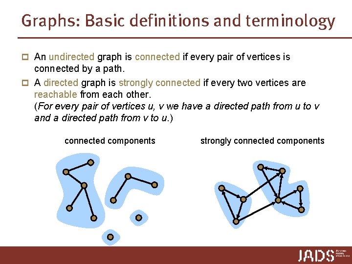
Graphs: Basic definitions and terminology p An undirected graph is connected if every pair of vertices is connected by a path. p A directed graph is strongly connected if every two vertices are reachable from each other. (For every pair of vertices u, v we have a directed path from u to v and a directed path from v to u. ) connected components strongly connected components

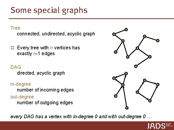
Some special graphs Tree connected, undirected, acyclic graph p Every tree with n vertices has exactly n-1 edges DAG directed, acyclic graph in-degree number of incoming edges out-degree number of outgoing edges every DAG has a vertex with in-degree 0 and with out-degree 0 …

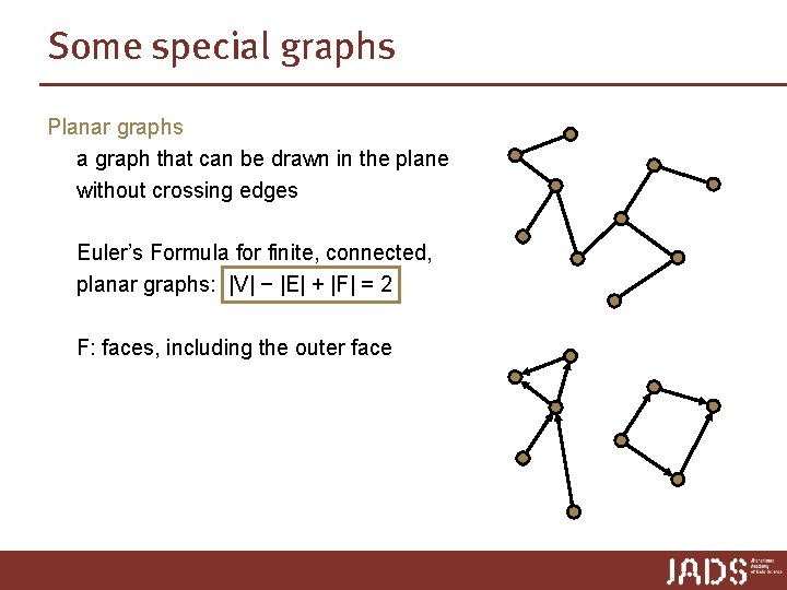
Some special graphs Planar graphs a graph that can be drawn in the plane without crossing edges Euler’s Formula for finite, connected, planar graphs: |V| − |E| + |F| = 2 F: faces, including the outer face

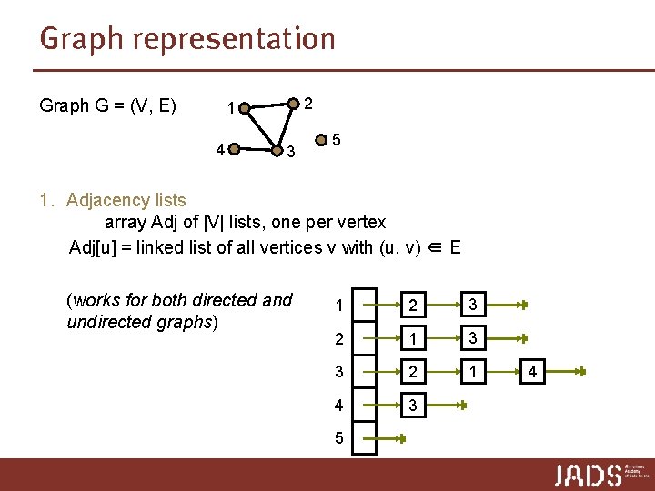
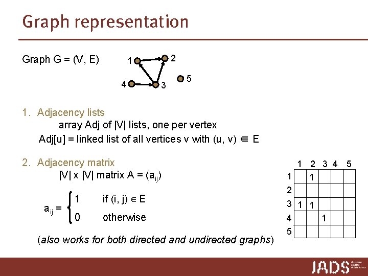
Graph representation Graph G = (V, E) 2 1 4 3 5 1. Adjacency lists array Adj of |V| lists, one per vertex Adj[u] = linked list of all vertices v with (u, v) ∈ E (works for both directed and undirected graphs) 1 2 3 2 1 3 3 2 1 4 3 5 4

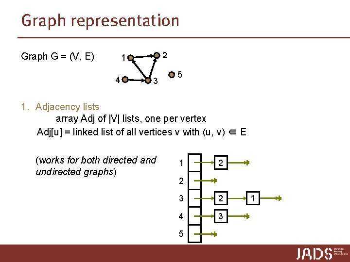
Graph representation Graph G = (V, E) 2 1 4 3 5 1. Adjacency lists array Adj of |V| lists, one per vertex Adj[u] = linked list of all vertices v with (u, v) ∈ E (works for both directed and undirected graphs) 1 2 2 3 2 4 3 5 1

Graph representation Graph G = (V, E) 2 1 4 3 5 1. Adjacency lists array Adj of |V| lists, one per vertex Adj[u] = linked list of all vertices v with (u, v) ∈ E 2. Adjacency matrix |V| matrix A = (aij) aij = 1 if (i, j) ∈ E 0 otherwise (also works for both directed and undirected graphs) 1 2 3 4 5 1 1 1 2 1 1 3 1 1 1 4 1 5

Graph representation Graph G = (V, E) 2 1 4 3 5 1. Adjacency lists array Adj of |V| lists, one per vertex Adj[u] = linked list of all vertices v with (u, v) ∈ E 2. Adjacency matrix |V| matrix A = (aij) aij = 1 if (i, j) ∈ E 0 otherwise (also works for both directed and undirected graphs) 1 2 3 4 5 1 1 2 3 1 1 4 5 1

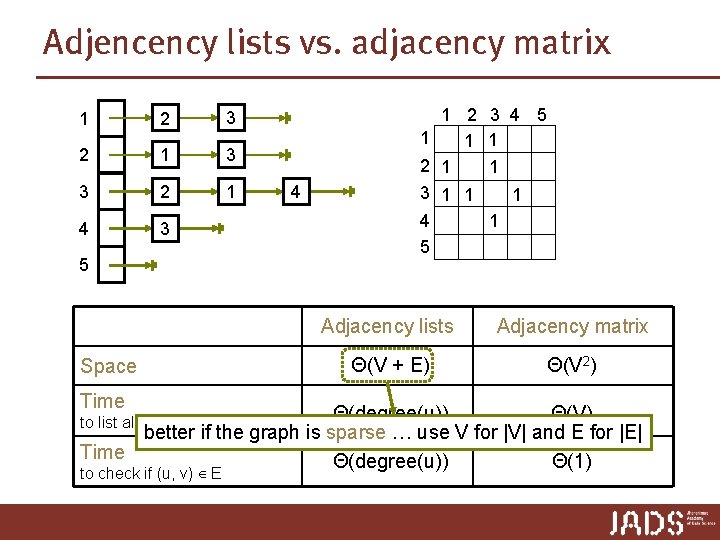
Adjencency lists vs. adjacency matrix 1 2 3 2 1 3 3 2 1 4 3 4 5 Space Time 1 2 3 4 5 1 1 1 2 1 1 3 1 1 1 4 1 5 Adjacency lists Adjacency matrix Θ(V + E) Θ(V 2) Θ(degree(u)) Θ(V) better if the graph is sparse … use V for |V| and E for |E| Time Θ(degree(u)) Θ(1) to list all vertices adjacent to u to check if (u, v) ∈ E

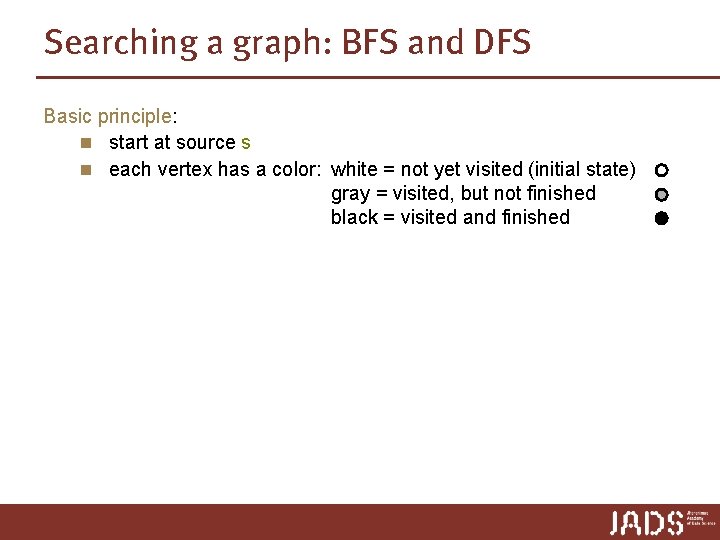
Searching a graph: BFS and DFS Basic principle: n start at source s n each vertex has a color: white = not yet visited (initial state) gray = visited, but not finished black = visited and finished

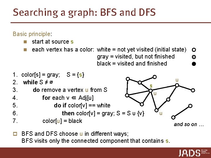
Searching a graph: BFS and DFS Basic principle: n start at source s n each vertex has a color: white = not yet visited (initial state) gray = visited, but not finished black = visited and finished 1. color[s] = gray; S = {s} 2. while S ≠ ∅ s 3. do remove a vertex u from S u 4. for each v ∈ Adj[u] 5. do if color[v] == white u 6. then color[v] = gray; S = S υ {v} 7. color[u] = black p BFS and DFS choose u in different ways; BFS visits only the connected component that contains s. u and so on …

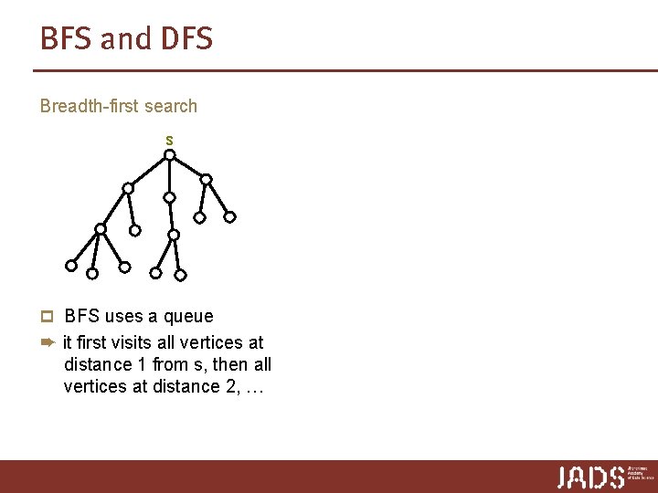
BFS and DFS Breadth-first search s p BFS uses a queue ➨ it first visits all vertices at distance 1 from s, then all vertices at distance 2, …

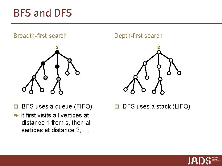
BFS and DFS Breadth-first search s p BFS uses a queue (FIFO) ➨ it first visits all vertices at distance 1 from s, then all vertices at distance 2, … Depth-first search s p DFS uses a stack (LIFO)

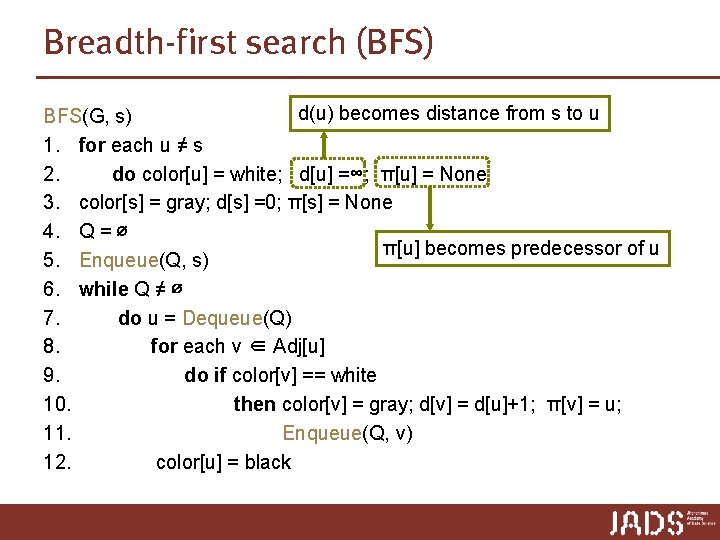
Breadth-first search (BFS) d(u) becomes distance from s to u BFS(G, s) 1. for each u ≠ s 2. do color[u] = white; d[u] =∞; π[u] = None 3. color[s] = gray; d[s] =0; π[s] = None 4. Q = ∅ π[u] becomes predecessor of u 5. Enqueue(Q, s) 6. while Q ≠ ∅ 7. do u = Dequeue(Q) 8. for each v ∈ Adj[u] 9. do if color[v] == white 10. then color[v] = gray; d[v] = d[u]+1; π[v] = u; 11. Enqueue(Q, v) 12. color[u] = black

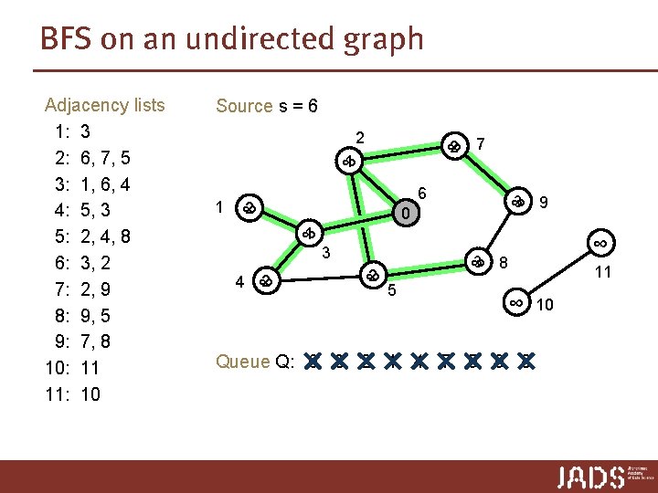
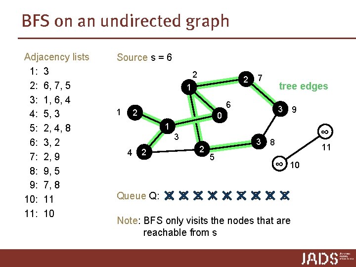
BFS on an undirected graph Adjacency lists 1: 3 2: 6, 7, 5 3: 1, 6, 4 4: 5, 3 5: 2, 4, 8 6: 3, 2 7: 2, 9 8: 9, 5 9: 7, 8 10: 11 11: 10 Source s = 6 2 2 ∞ 1 6 2 ∞ 3 ∞ 0 1 ∞ 4 7 2 ∞ 3 ∞ 5 9 ∞ 8 11 ∞ Queue Q: 6 3 2 1 4 7 5 9 8 10

BFS on an undirected graph Adjacency lists 1: 3 2: 6, 7, 5 3: 1, 6, 4 4: 5, 3 5: 2, 4, 8 6: 3, 2 7: 2, 9 8: 9, 5 9: 7, 8 10: 11 11: 10 Source s = 6 2 2 1 ∞ 1 7 6 2 tree edges 3 ∞ 0 9 1 3 4 2 2 ∞ 3 8 5 11 ∞ 10 Queue Q: 6 3 2 1 4 7 5 9 8 Note: BFS only visits the nodes that are reachable from s

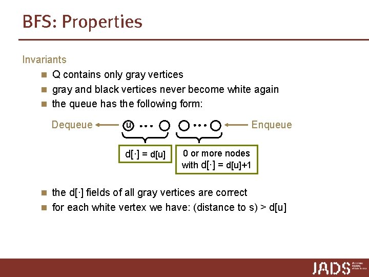
BFS: Properties Invariants n Q contains only gray vertices n gray and black vertices never become white again n the queue has the following form: Dequeue Enqueue u d[∙] = d[u] 0 or more nodes with d[∙] = d[u]+1 n the d[∙] fields of all gray vertices are correct n for each white vertex we have: (distance to s) > d[u]

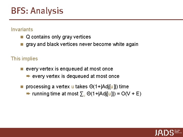
BFS: Analysis Invariants n Q contains only gray vertices n gray and black vertices never become white again This implies n every vertex is enqueued at most once ➨ every vertex is dequeued at most once n processing a vertex u takes Θ(1+|Adj[u]|) time ➨ running time at most ∑u Θ(1+|Adj[u]|) = O(V + E)

BFS: Properties After BFS has been run from a source s on a graph G we have n each vertex u that is reachable from s has been visited n for each vertex u we have d[u] = distance to s n if d[u] < ∞, then there is a shortest path from s to u that is a shortest path from s to π[u] followed by the edge (π[u], u) Proof: follows from the invariants BFS computes a shortest path tree (breadth-first tree) on the connected component of G containing s, consisting of edges (u, v) such that u is gray and v is white when (u, v) is explored.

Depth-first search (DFS) DFS(G) 1. for each u ∈ V 2. do color[u] = white; π[u] = None time = global timestamp for 3. time = 0 discovering and finishing vertices 4. for each u ∈ V 5. do if color[u] == white then DFS-Visit(u) 1. color[u] = gray; d[u] =time; time = time + 1 2. for each v ∈ Adj[u] 3. do if color[v] == white 4. then π[v] = u; DFS-Visit(v) 5. color[u] = black; f[u] =time; time = time + 1 d[u] = discovery time f[u] = finishing time

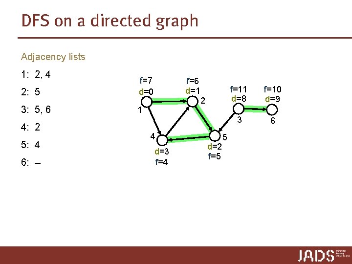
DFS on a directed graph Adjacency lists 1: 2, 4 2: 5 f=7 d=0 3: 5, 6 1 4: 2 5: 4 6: -- f=6 d=1 2 4 d=3 f=4 d=2 f=5 5 f=11 d=8 f=10 d=9 3 6

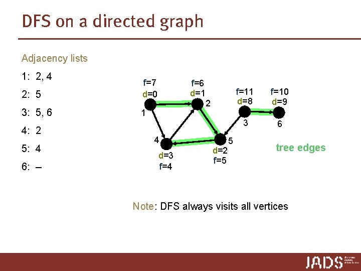
DFS on a directed graph Adjacency lists 1: 2, 4 2: 5 f=7 d=0 3: 5, 6 1 4: 2 5: 4 6: -- f=6 d=1 2 4 d=3 f=4 d=2 f=5 5 f=11 d=8 f=10 d=9 3 6 tree edges Note: DFS always visits all vertices

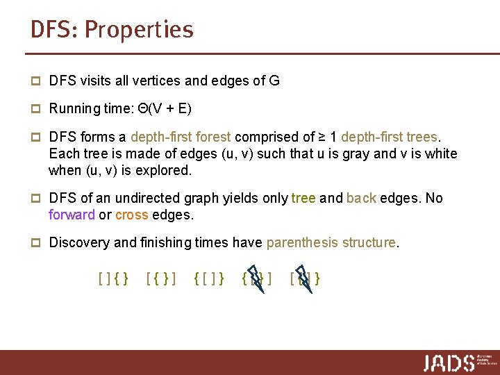
DFS: Properties p DFS visits all vertices and edges of G p Running time: Θ(V + E) p DFS forms a depth-first forest comprised of ≥ 1 depth-first trees. Each tree is made of edges (u, v) such that u is gray and v is white when (u, v) is explored.

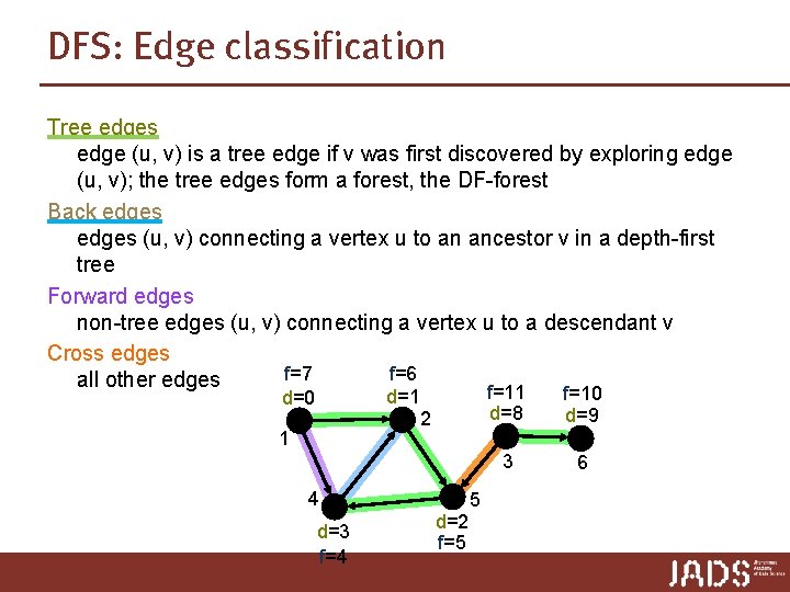
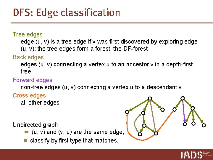
DFS: Edge classification Tree edges edge (u, v) is a tree edge if v was first discovered by exploring edge (u, v); the tree edges form a forest, the DF-forest Back edges (u, v) connecting a vertex u to an ancestor v in a depth-first tree Forward edges non-tree edges (u, v) connecting a vertex u to a descendant v Cross edges f=7 f=6 all other edges d=1 2 d=0 1 4 d=3 f=4 d=2 f=5 5 f=11 d=8 f=10 d=9 3 6

DFS: Edge classification Tree edges edge (u, v) is a tree edge if v was first discovered by exploring edge (u, v); the tree edges form a forest, the DF-forest Back edges (u, v) connecting a vertex u to an ancestor v in a depth-first tree Forward edges non-tree edges (u, v) connecting a vertex u to a descendant v Cross edges all other edges Undirected graph ➨ (u, v) and (v, u) are the same edge; n classify by first type that matches.

DFS: Properties p DFS visits all vertices and edges of G p Running time: Θ(V + E) p DFS forms a depth-first forest comprised of ≥ 1 depth-first trees. Each tree is made of edges (u, v) such that u is gray and v is white when (u, v) is explored. p DFS of an undirected graph yields only tree and back edges. No forward or cross edges. p Discovery and finishing times have parenthesis structure. []{} [{}] {[]} {[}] [{]}

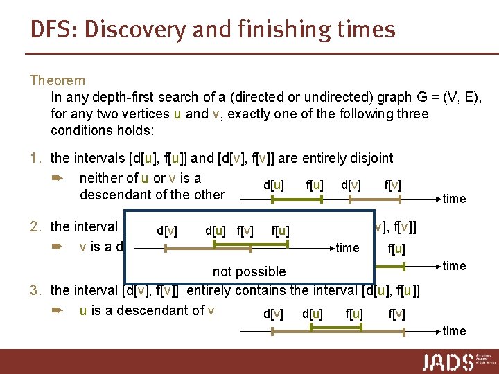
DFS: Discovery and finishing times Theorem In any depth-first search of a (directed or undirected) graph G = (V, E), for any two vertices u and v, exactly one of the following three conditions holds: 1. the intervals [d[u], f[u]] and [d[v], f[v]] are entirely disjoint ➨ neither of u or v is a d[u] f[u] d[v] f[v] descendant of the other time 2. the interval [d[u], d[v] f[u]] entirely d[u] contains f[v] f[u]the interval [d[v], f[v]] ➨ v is a descendant of u d[u] d[v] time f[v] f[u] not possible 3. the interval [d[v], f[v]] entirely contains the interval [d[u], f[u]] ➨ u is a descendant of v d[v] d[u] f[v] time

DFS: Discovery and finishing times Proof (sketch): n assume d[u] < d[v] case 1: v is discovered in a recursive call from u ➨ v becomes a descendant of u recursive calls are finished before u itself is finished ➨ f[v] < f[u] case 2: v is not discovered in a recursive call from u ➨ v is not reachable from u and not one of u’s descendants ➨ v is discovered only after u is finished ➨ f[u] < d[v] ➨ u cannot become a descendant of v since it is already discovered ■

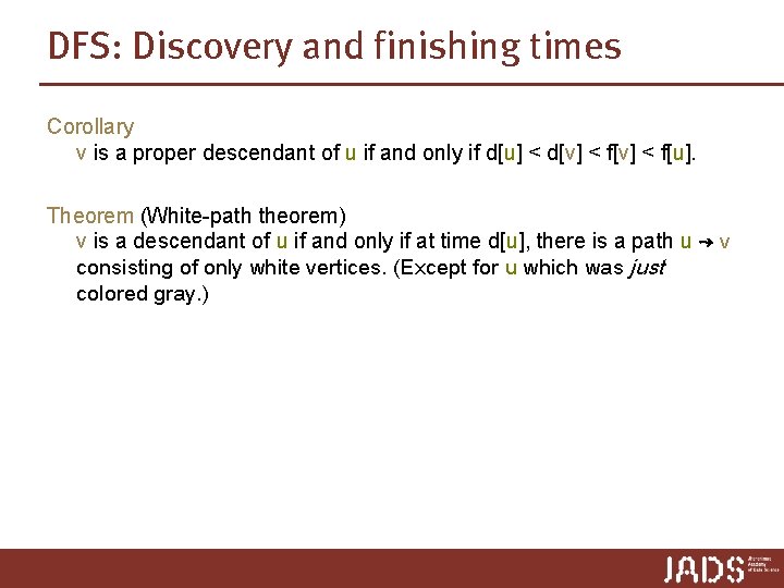
DFS: Discovery and finishing times Corollary v is a proper descendant of u if and only if d[u] < d[v] < f[u]. Theorem (White-path theorem) v is a descendant of u if and only if at time d[u], there is a path u ↝ v consisting of only white vertices. (Except for u which was just colored gray. )

Topological sort Using depth-first search …

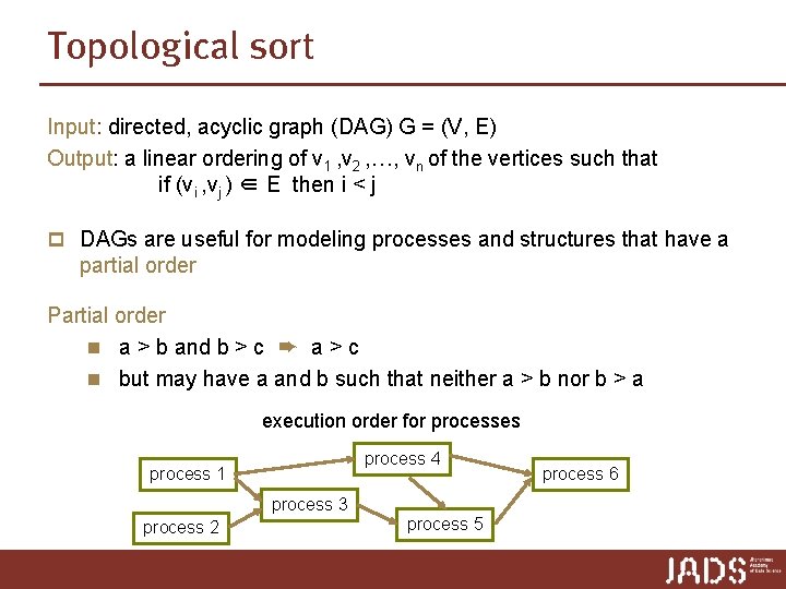
Topological sort Input: directed, acyclic graph (DAG) G = (V, E) Output: a linear ordering of v 1 , v 2 , …, vn of the vertices such that if (vi , vj ) ∈ E then i < j p DAGs are useful for modeling processes and structures that have a partial order Partial order n a > b and b > c ➨ a > c n but may have a and b such that neither a > b nor b > a execution order for processes process 4 process 1 process 3 process 2 process 5 process 6

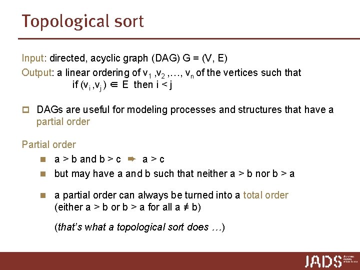
Topological sort Input: directed, acyclic graph (DAG) G = (V, E) Output: a linear ordering of v 1 , v 2 , …, vn of the vertices such that if (vi , vj ) ∈ E then i < j p DAGs are useful for modeling processes and structures that have a partial order Partial order n a > b and b > c ➨ a > c n but may have a and b such that neither a > b nor b > a n a partial order can always be turned into a total order (either a > b or b > a for all a ≠ b) (that’s what a topological sort does …)

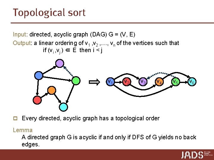
Topological sort Input: directed, acyclic graph (DAG) G = (V, E) Output: a linear ordering of v 1 , v 2 , …, vn of the vertices such that if (vi , vj ) ∈ E then i < j v 1 v 2 v 3 v 4 v 5 v 6 p Every directed, acyclic graph has a topological order Lemma A directed graph G is acyclic if and only if DFS of G yields no back edges.

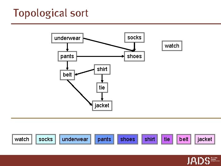
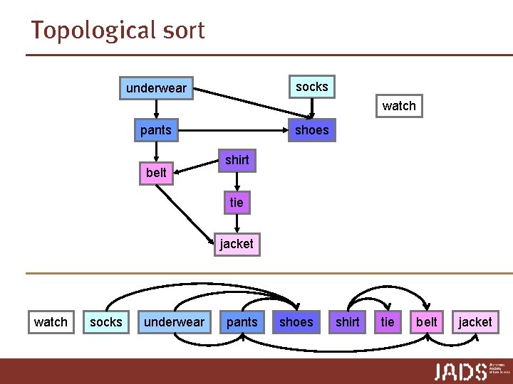
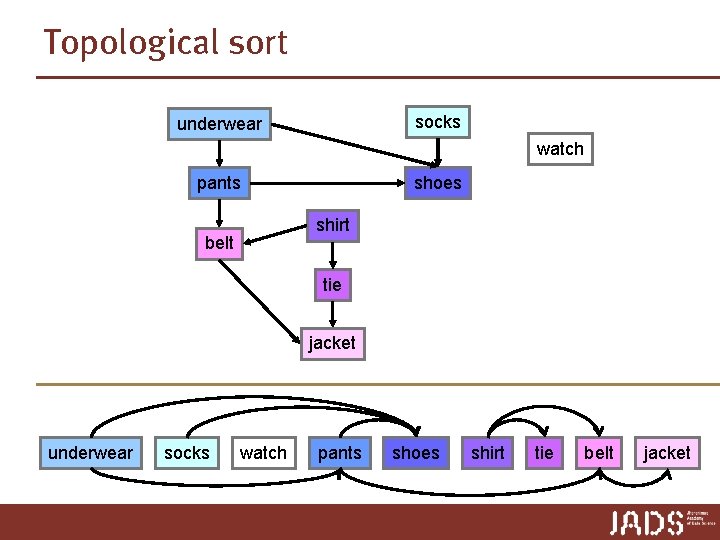
Topological sort socks underwear watch pants belt shoes shirt tie jacket watch socks underwear pants shoes shirt tie belt jacket

Topological sort socks underwear watch pants belt shoes shirt tie jacket watch socks underwear pants shoes shirt tie belt jacket

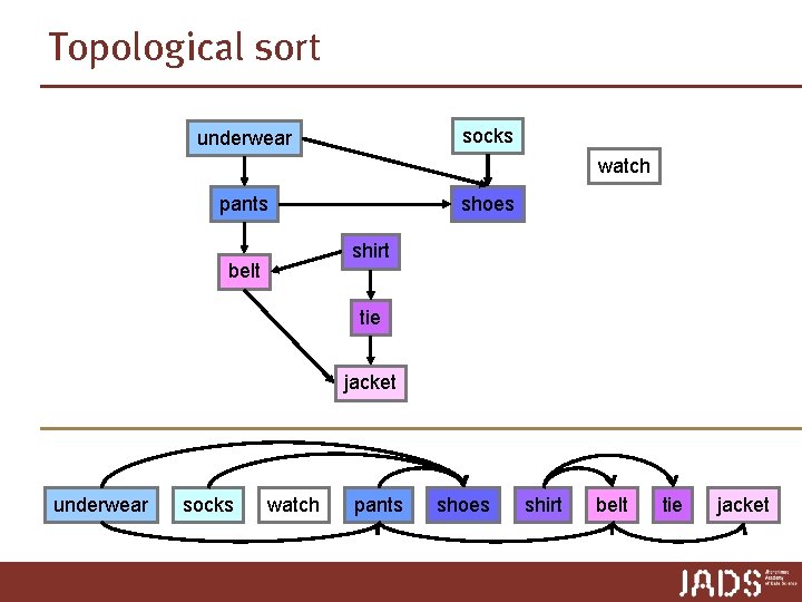
Topological sort socks underwear watch pants shoes shirt belt tie jacket underwear socks watch pants shoes shirt tie belt jacket

Topological sort socks underwear watch pants shoes shirt belt tie jacket underwear socks watch pants shoes shirt belt tie jacket

Topological sort Topological. Sort(V, E) 1. call DFS(V, E) to compute finishing time f[v] for all v ∈ E 2. output vertices in order of decreasing finishing time 10 15 socks underwear 11 14 5 6 pants belt shoes 0 shirt tie jacket 7 1 4 2 3 16 17 12 13 watch 8 9

Topological sort Topological. Sort(V, E) 1. call DFS(V, E) to compute finishing time f[v] for all v ∈ E 2. output vertices in order of decreasing finishing time socks 16 10 17 15 11 underwear 14 pants shoes 12 13 watch jacket 2 3 tie 1 5 4 6 belt shirt 0 7 8 9

Topological sort Topological. Sort(V, E) 1. call DFS(V, E) to compute finishing time f[v] for all v ∈ E 2. output vertices in order of decreasing finishing time Lemma Topological. Sort(V, E) produces a topological sort of a directed acyclic graph G = (V, E).

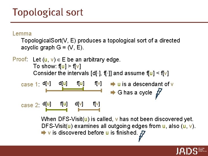
Topological sort Lemma Topological. Sort(V, E) produces a topological sort of a directed acyclic graph G = (V, E). Proof: Let (u, v) ∈ E be an arbitrary edge. To show: f[u] > f[v] Consider the intervals [d[∙], f[∙]] and assume f[u] < f[v] case 1: d[v] d[u] f[u] case 2: d[u] f[u] d[v] f[v] ➨ u is a descendant of v ➨ G has a cycle f[v] When DFS-Visit(u) is called, v has not been discovered yet. DFS-Visit(u) examines all outgoing edges from u, also (u, v). ➨ v is discovered before u is finished.

Topological sort Lemma Topological. Sort(V, E) produces a topological sort of a directed acyclic graph G = (V, E). Running time? n we do not need to sort by finishing times n just output vertices as they are finished ➨ Θ(V + E) for DFS and Θ(V) for output ➨ Θ(V + E)

Recap Today p Graphs p Graph representations: adjacency list, adjacency matrix p BFS and DFS p Topological sorting